
Videos
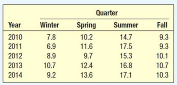
The quarterly production of pine lumber, in millions of board feet, by Northwest Lumber for 2010 through 2014 is:
- a. Determine the typical seasonal pattern for the production data using the ratio-to-moving-average method.
- b. Interpret the pattern.
- c. Deseasonalize the data and determine the linear trend equation.
- d. Project the seasonally adjusted production for the four quarters of 2015.
a.
Obtain the typical seasonal patterns for the production data using the ratio-to-moving-average method.
Answer to Problem 28CE
The typical seasonal patterns for sales are 0.7549, 0.9913, 1.4043, and 0.8495.
Explanation of Solution
Four-year moving average:
Centered moving average:
Specific seasonal index:
| Year | Quarter | Board ft Millions |
Four-quarter moving average |
Centered Moving average | Specific seasonal |
| 2010 | Winter | 7.8 | |||
| Spring | 10.2 | ||||
| Summer | 14.7 | 10.3875 | 1.41516 | ||
| Fall | 9.3 | 10.5 | 10.45 | 0.88995 | |
| 2011 | Winter | 6.9 | 10.275 | 10.975 | 0.6287 |
| Spring | 11.6 | 10.625 | 11.325 | 1.02428 | |
| Summer | 17.5 | 11.325 | 11.575 | 1.51188 | |
| Fall | 9.3 | 11.325 | 11.5875 | 0.80259 | |
| 2012 | Winter | 8.9 | 11.825 | 11.075 | 0.80361 |
| Spring | 9.7 | 11.35 | 10.9 | 0.88991 | |
| Summer | 15.3 | 10.8 | 11.225 | 1.36303 | |
| Fall | 10.1 | 11 | 11.7875 | 0.85684 | |
| 2013 | Winter | 10.7 | 11.45 | 12.3125 | 0.86904 |
| Spring | 12.4 | 12.125 | 12.575 | 0.98608 | |
| Summer | 16.8 | 12.5 | 12.4625 | 1.34804 | |
| Fall | 10.7 | 12.65 | 12.425 | 0.86117 | |
| 2014 | Winter | 9.2 | 12.275 | 12.6125 | 0.72944 |
| Spring | 13.6 | 12.575 | 12.6 | 1.07937 | |
| Summer | 17.1 | 12.65 | |||
| Fall | 10.3 | 12.55 |
The quarterly indexes are as follows:
| Winter | Spring | Summer | Fall | |
| 2010 | 1.415162 | 0.889952 | ||
| 2011 | 0.628702 | 1.024283 | 1.511879 | 0.802589 |
| 2012 | 0.803612 | 0.889908 | 1.363029 | 0.85684 |
| 2013 | 0.869036 | 0.986083 | 1.348044 | 0.861167 |
| 2014 | 0.729435 | 1.079365 | ||
| Mean | 0.757696 | 0.99491 | 1.409529 | 0.852637 |
Typical seasonal index:
Here,
Therefore, the following is obtained:
The typical seasonal indexes are as follows:
| Winter | Spring | Summer | Fall | |
| 2010 | 1.415162 | 0.889952 | ||
| 2011 | 0.628702 | 1.024283 | 1.511879 | 0.802589 |
| 2012 | 0.803612 | 0.889908 | 1.363029 | 0.85684 |
| 2013 | 0.869036 | 0.986083 | 1.348044 | 0.861167 |
| 2014 | 0.729435 | 1.079365 | ||
| Mean | 0.757696 | 0.99491 | 1.409529 | 0.852637 |
| Typical Index | 0.7549 | 0.9913 | 1.4043 | 0.8495 |
b.
Interpret the typical seasonal pattern.
Explanation of Solution
The typical seasonal index for the summer quarter is 1.4043, which is the largest compared to the other three quarters. That is, the production is the largest in the third quarter and moreover, it represents above the average quarters because the corresponding seasonal index is greater than 1. The winter, spring, and fall quarters represent below the average quarters because seasonal indexes for the three quarters are less than 1.
c.
Determine the trend equation.
Answer to Problem 28CE
The trend equation is
Explanation of Solution
Calculation:
Deseasonalization:
| Board ft Millions | Typical Seasonal Index | Deseasonalized production |
| 7.8 | 0.7549 | 10.33249437 |
| 10.2 | 0.9913 | 10.28951881 |
| 14.7 | 1.4043 | 10.46784875 |
| 9.3 | 0.8495 | 10.94761624 |
| 6.9 | 0.7549 | 9.140283481 |
| 11.6 | 0.9913 | 11.70180571 |
| 17.5 | 1.4043 | 12.4617247 |
| 9.3 | 0.8495 | 10.94761624 |
| 8.9 | 0.7549 | 11.78964101 |
| 9.7 | 0.9913 | 9.785130637 |
| 15.3 | 1.4043 | 10.89510788 |
| 10.1 | 0.8495 | 11.88934667 |
| 10.7 | 0.7549 | 14.17406279 |
| 12.4 | 0.9913 | 12.50882679 |
| 16.8 | 1.4043 | 11.96325571 |
| 10.7 | 0.8495 | 12.5956445 |
| 9.2 | 0.7549 | 12.18704464 |
| 13.6 | 0.9913 | 13.71935842 |
| 17.1 | 1.4043 | 12.17688528 |
| 10.3 | 0.8495 | 12.12477928 |
Assign t value as 1 for the first quarter of 2010, 2 for the second quarter of 2010, and so on.
Step-by-step procedure to obtain the regression using the Excel:
- Enter the data for Deseasonalized production and t in Excel sheet.
- Go to Data Menu.
- Click on Data Analysis.
- Select Regression and click on OK.
- Select the column of Deseasonalized production under Input Y Range.
- Select the column of t under Input X Range.
- Click on OK.
Output for the regression obtained using the Excel is as follows:
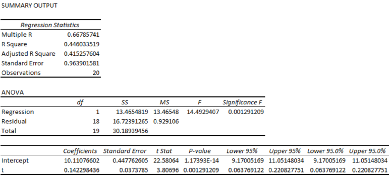
From the Excel output, the regression equation is
d.
Find the seasonally adjusted production for the four quarters of 2017.
Answer to Problem 28CE
The seasonally adjusted production for the four quarters of 2017 are 9.8884, 13.1261, 18.7946, and 11.4903.
Explanation of Solution
From the output, the regression equation is
The t value for the first quarter of 2017 is 21.
The t value for the second quarter of 2017 is 22.
The t value for the third quarter of 2017 is 23.
The t value for the fourth quarter of 2017 is 24.
Seasonally adjusted forecast:
| Estimated Visitors | Seasonal Index | |
| 13.0990 | 0.7549 | 9.8884 |
| 13.2413 | 0.9913 | 13.1261 |
| 13.3836 | 1.4043 | 18.7946 |
| 13.5259 | 0.8495 | 11.4903 |
Want to see more full solutions like this?
Chapter 18 Solutions
STAT TECHNIQUES IN BUSI 2370 >CI<


 Big Ideas Math A Bridge To Success Algebra 1: Stu...AlgebraISBN:9781680331141Author:HOUGHTON MIFFLIN HARCOURTPublisher:Houghton Mifflin Harcourt
 Glencoe Algebra 1, Student Edition, 9780079039897...AlgebraISBN:9780079039897Author:CarterPublisher:McGraw Hill
 Trigonometry (MindTap Course List)TrigonometryISBN:9781337278461Author:Ron LarsonPublisher:Cengage Learning
 Holt Mcdougal Larson Pre-algebra: Student Edition...AlgebraISBN:9780547587776Author:HOLT MCDOUGALPublisher:HOLT MCDOUGAL
 Functions and Change: A Modeling Approach to Coll...AlgebraISBN:9781337111348Author:Bruce Crauder, Benny Evans, Alan NoellPublisher:Cengage Learning