
Videos
For each of the determinants of
The impact of various factors on the demand, supply, and equilibrium price of hybrid gasoline-electric vehicles like Toyota Prius with the help of given supply and demand function.
Explanation of Solution
The demand curve is the graphical representation of quantity demanded by a consumer at a given price level. The changes in quantity demanded on the demand curve can be determined in two ways.
- Movement along the demand curve: this happens when the price of commodity change while keeping another factor constant. A rise in price leads to an upward movement along the demand curve whereas, when the price falls it leads to a downward movement along the demand curve.
- The shift in the demand curve: when factors other than price changes, demand curve shift either right or left
The demand function for Toyota prius can be expressed as:
Here, QD = quantity demanded of Toyota Prius,
P = price of Toyota prius,
PS = price of Nissan leaf, it is substitutes of Toyota prius,
PC = price of gasoline, which is complementary good for Toyota prius,
Y = income of consumers
A = advertising and promotion expenditures by Toyota
AC = competitors’ advertising and promotion expenditures
N = size of the potential target market
CP = consumer tastes and preferences for Toyota,
PE = expected future price appreciation or depreciation Toyota prius,
TA = purchase adjustment time period
T/S = taxes or subsidies on Toyota.
As demand for good increases (decreases), it will lead to increase (decrease) the equilibrium price of that good.
These are the factors that can impact the demand for Toyota prius (TP) in following manner:
| Factors | Result of change in factors | Equilibrium price: increase or decrease. |
| Increase (decrease) in price of Toyota prius | Decrease (increase) in quantity demanded for TP. | - |
| Increase (decrease) in price of Nissan leaf | Increase (decrease) in demand for TP. | Increase (decrease) in equilibrium price of TP. |
| Increase (decrease) in price of gasoline | Decrease (increase) in demand for TP. | Decrease (increase) in equilibrium price of TP. |
| Increase (decrease) in income of consumers | Increase (decrease) in demand for TP. | Increase (decrease) in equilibrium price of TP. |
| Increase (decrease) in advertising and promotion expenditures by Toyota | Increase (decrease) in demand for TP. | Increase (decrease) in equilibrium price of TP. |
| Increase (decrease) in competitors’ advertising and promotion expenditures | Decrease (increase) in demand for TP. | Decrease (increase) in equilibrium price of TP. |
| Increase (decrease) in size of the potential target market | Increase (decrease) in demand for TP. | Increase (decrease) in equilibrium price of TP. |
| Increase (decrease) in consumer tastes and preferences for Toyota | Increase (decrease) in demand for TP. | Increase (decrease) in equilibrium price of TP. |
| Increase (decrease) in expected future price appreciation or depreciation Toyota prius | Increase (decrease) in demand for TP. | Increase (decrease) in equilibrium price of TP. |
| Increase (decrease) in purchase adjustment time period | Increase (decrease) in demand for TP. | Increase (decrease) in equilibrium price of TP. |
| Increase (decrease) in taxes or subsidies on Toyota. | Decrease (increase) in demand for TP. Because of tax, price of TP rises and as a result demand will fall. | Decrease (increase) in equilibrium price of TP. |
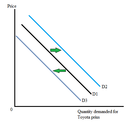
With the help of following graph, the increase and decrease in demand for TP can be seen. As demand for TP increases, the demand curve shifts to the right from D1 to D2. And as demand for TP fall, the demand curve shifts to the left from D1 to D3.
The supply curve is the graphical representation of quantity supplied by a producer at a given price level.
The supply function for Toyota prius (TP) can be expressed as:
Here, Qs = quantity supplied of TP
P = price of the TP
PI = price of inputs like sheet metal
PUI = price of unused substitute inputs like fiberglass
T = technological improvements
EE = entry or exit of other auto sellers
F = accidental supply interruptions from fires, floods, etc.
RC = costs of regulatory compliance
PE = expected (future) changes in price
TA = adjustment time period
T/S = taxes or subsidies
As supply of good increases (decreases), it will lead to decrease (increase) the equilibrium price of that good.
These are the factors that can impact the demand for Toyota prius (TP) in following manner:
| Factors | Result of change in factors | Equilibrium price: increase or decrease. |
| Increase (decrease) in price of Toyota prius | Increase (decrease) in quantity supplied for TP. | Decrease (increase) in equilibrium price of TP. |
| Increase (decrease) in price of inputs like sheet metal | Decrease (increase) in supply of TP. | Increase (decrease) in equilibrium price of TP. |
| Increase (decrease) in price of unused substitute inputs like fiberglass | Decrease (increase) in supply of TP. | Increase (decrease) in equilibrium price of TP. |
| Increase (decrease) in technological improvements | Increase (decrease) in supply of TP. | Decrease (increase) in equilibrium price of TP. |
| Increase (decrease) in entry or exit of other auto sellers | Increase (decrease) in supply of TP. | Decrease (increase) in equilibrium price of TP. |
| Increase (decrease) in accidental supply interruptions from fires, floods, etc. | Decrease (increase) in supply of TP. | Increase (decrease) in equilibrium price of TP. |
| Increase (decrease) in costs of regulatory compliance | Decrease (increase) in supply of TP. | Increase (decrease) in equilibrium price of TP. |
| Increase (decrease) in expected (future) changes in price | Decrease (increase) in supply of TP. | Increase (decrease) in equilibrium price of TP. |
| Increase (decrease) in adjustment time period | Increase (decrease) in supply of TP. | Decrease (increase) in equilibrium price of TP. |
| Increase (decrease) in taxes or subsidies on Toyota. | Decrease (increase) in supply of TP. | Increase (decrease) in equilibrium price of TP. |
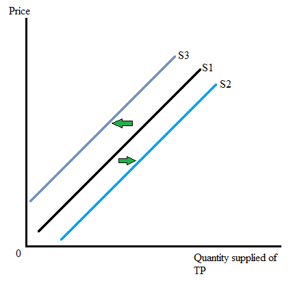
With the help of following graph, the increase and decrease in supply of TP can be seen. As supply of TP increases, the supply curve shifts to the right from S1 to S2. And as supply of TP fall, the supply curve shifts to the left from S1 to S3.
Want to see more full solutions like this?
Chapter 2 Solutions
Managerial Economics: Applications, Strategies and Tactics (MindTap Course List)


- (Calculating Price Elasticity of Demand) Suppose that 50 units of a good are demanded at a price of Si per unit. A reduction in price to $0.20 results in an increase in quantity demanded to 70 units. Using the midpoint formula, show that these data yield a price elasticity of 0.25. By what percentage would a 10 percent rise in the price reduce the quantity demanded, assuming price elasticity remains constant along the demand curve?arrow_forwardIf automobiles and gasoline are complements, then their cross-elasticity coefficient is a. strictly greater than 1. b. positive. c. equal to zero. d. negative.arrow_forwardFind the equilibrium quantity and equilibrium price for the commodity whose supply and demand functions are given. Supply: p= q^2+ 20q Demand: p= −2q^2+ 10q+ 11,400arrow_forward
- In this exercise, you will analyze the supply-demand equilibrium of a city under some special simplifying assumptions about land use. The assumptions are: (i) all dwellings must contain exactly 1,500 square feet of fl oor space, regardless of location, and (ii) apartment complexes must contain exactly 15,000 square feet of fl oor space per square block of land area. These land-use restrictions, which are imposed by a zoning authority, mean that dwelling sizes and building heights do not vary with distance to the central business district, as in the model from chapter 2. Distance is measured in blocks. Suppose that income per household equals $25,000 per year. It is convenient to measure money amounts in thousands of dollars, so this means that y = 25, where y is income. Next suppose that the commuting cost parameter t equals 0.01. This means that a person living ten blocks from the CBD will spend 0.01 × 10 = 0.1 per year (in other words, $100) getting to work. The consumer ’ s budget…arrow_forwardThe demand function for fountain pens last week is given as Qd=14-2P. If two fountain pens are sold at $4.00 each at the end of this week: Formulate the supply function. Find the equilibrium price. Find the equilibrium quantity.arrow_forwardIn a given market, there are three demanders of a good with Qd¹+P=12, P=10-2Qd² and Qd³=10-P as their respective demand functions, obtain the market demand for the good and determine the market Quantity demanded when the price of the good is Gh4.arrow_forward
- Which of the following graphs best describes the expected changes in the market for flights from Oakland to Mauai if consumers' airlines cut back the number of daily flights while at the same time the state of Hawaii does not allow tourists from leaving their hotel rooms for the first two weeks of their stay due to concerns over COVID-19?arrow_forwardCalculate the equilibrium price when the demand equation is given as:- 20P - 18 And the supply equation is :- 10P + 32arrow_forwardSuppose the estimated supply function for avocados is given by QS = 48 + 15p – 10pf , where pf is the price of fertilizer. The estimated demand for avocados is given by Qd = 233 - 40p + 5pt , where pt is the price of tomatoes per pound. Solve for the initial equilibrium price and quantity of avocados if the price of fertilizer, pf ,is equal to $0.35 per lb. and price of tomatoes, pt, is equal to $0.80 per lb. Solve for the new equilibrium price and quantity of avocados if the price of fertilizer, pf , increases to $0.90 per lb. and price of tomatoes, pt, remains $0.80 per lb. Use these equilibrium values from parts a. and b. to solve for the price elasticity of demand for avocados. Given your calculations, are avocados elastic, inelastic or unit-elastic? Have total expenditures on avocados increased, decreased, or not changed as a result of the change in the price of fertilizer?arrow_forward
 Managerial Economics: Applications, Strategies an...EconomicsISBN:9781305506381Author:James R. McGuigan, R. Charles Moyer, Frederick H.deB. HarrisPublisher:Cengage Learning
 Microeconomics: Private and Public Choice (MindTa...EconomicsISBN:9781305506893Author:James D. Gwartney, Richard L. Stroup, Russell S. Sobel, David A. MacphersonPublisher:Cengage Learning
 Macroeconomics: Private and Public Choice (MindTa...EconomicsISBN:9781305506756Author:James D. Gwartney, Richard L. Stroup, Russell S. Sobel, David A. MacphersonPublisher:Cengage Learning
 Economics: Private and Public Choice (MindTap Cou...EconomicsISBN:9781305506725Author:James D. Gwartney, Richard L. Stroup, Russell S. Sobel, David A. MacphersonPublisher:Cengage Learning
