Chapter 2, Problem 2.58SE

a.

To determine

Explain the data and count the number of observations that fall into the given intervals.

Answer to Problem 2.58SE

  $82\%$ of data values lie in between $0.697$ and $16.04$ .

  $94\%$ of data values lie in between $-6.97$ and $23.7$ .

  $98\%$ of data values lie in between $-14.6$ and $31.38$ .

Explanation of Solution

Given:

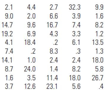
The data shows the lengths of time between the onset of a particular illness and its recurrence were recorded.

  

Calculation:

Given: the given intervals are $\overline{x}\pm s,\overline{x}\pm 2s,\text{and}\overline{x}\pm 3s$ .

Arrange the data values from smallest to largest.

  $\begin{array}{l}0.2,0.2,0.3,0.4,1,1.2,1.3,1.4,1.6,1.6,2,2.1,2.4,2.4,2.7,3.3,3.5,3.7,\\ 3.9,4.1,4.3,4.4,5.6,5.8,6.1,6.6,6.9,7.4,7.4,8.2,8.2,8.3,8.7,9,9.6,9.9,\\ 11.4,12.6,13.5,14.1,14.7,16.7,18,18,18.4,19.2,23.1,24,26.7,32.3\end{array}$

  $\text{Mean}=\frac{\text{sum}\text{of}\text{all}\text{values}}{\text{total}\text{number}\text{of}\text{values}}$

  $\begin{array}{l}\overline{x}=\frac{{\displaystyle \sum _{i=1}^n{x}_i}}{n}\\ =\frac{\begin{array}{l}0.2+0.2+0.3+0.4+1+1.2+1.3+1.4+1.6+1.6+2+2.1+2.4+2.4+2.7+3.3+3.5+3.7+\\ 3.9+4.1+4.3+4.4+5.6+5.8+6.1+6.6+6.9+7.4+7.4+8.2+8.2+8.3+8.7+9+9.6+9.9+\\ 11.4+12.6+13.5+14.1+14.7+16.7+18+18+18.4+19.2+23.1+24+26.7+32.3\end{array}}{\text{50}}\\ =\frac{418.4}{50}\\ \approx 8.37\end{array}$ find the sample variance $s^2=\frac{{\displaystyle \sum x_i{}^2-\frac{{\left({\displaystyle \sum x_i}\right)}^2}{n}}}{n-1}$

  $n=$ total number of data values.

  $n=25$

  $\begin{array}{l}{\displaystyle \sum x_i}=0.2+0.2+0.3+0.4+1+1.2+1.3+1.4+1.6+1.6+2+2.1+2.4+2.4+2.7+3.3+3.5+3.7+\\ 3.9+4.1+4.3+4.4+5.6+5.8+6.1+6.6+6.9+7.4+7.4+8.2+8.2+8.3+8.7+9+9.6+9.9+\\ 11.4+12.6+13.5+14.1+14.7+16.7+18+18+18.4+19.2+23.1+24+26.7+32.3=418.4\\ {\displaystyle \sum x_i{}^2}={0.2}^2+{0.2}^2+{0.3}^2+{0.4}^2+1^2+{1.2}^2+{1.3}^2+{1.4}^2+{1.6}^2+{1.6}^2+2^2+{2.1}^2+{2.4}^2+{2.4}^2+{2.7}^2+{3.3}^2+{3.5}^2+{3.7}^2+\\ {3.9}^2+{4.1}^2+{4.3}^2+{4.4}^2+{5.6}^2+{5.8}^2+{6.1}^2+{6.6}^2+{6.9}^2+{7.4}^2+{7.4}^2+{8.2}^2+{8.2}^2+{8.3}^2+{8.7}^2+9^2+{9.6}^2+{9.9}^2+\\ {11.4}^2+{12.6}^2+{13.5}^2+{14.1}^2+{14.7}^2+{16.7}^2+{18}^2+{18}^2+{18.4}^2+{19.2}^2+{23.1}^2+{24}^2+{26.7}^2+{32.3}^2=6384.34\end{array}$

  $\begin{array}{l}{s}^2=\frac{6384.34-\frac{{418.4}^2}{50}}{50-1}\\ =\frac{6384.34-\frac{{418.4}^2}{50}}{49}\\ \approx 58.8\end{array}$

  $s=\sqrt{58.8}=7.67$

Calculate $\overline{x}\pm s,\overline{x}\pm 2s,\text{and}\overline{x}\pm 3s$ .

  $\begin{array}{l}\overline{x}-3s=8.37-3\left(7.67\right)=-14.6\\ \overline{x}-2s=8.37-2\left(7.67\right)=-6.97\\ \overline{x}-s=8.37-7.67=0.697\\ \overline{x}+3s=8.37+3\left(7.67\right)=31.38\\ \overline{x}+2s=8.37+2\left(7.67\right)=23.7\\ \overline{x}+s=8.37+7.67=16.04\end{array}$

  $41$ of the $50$ data values lie in between $0.697$ and $16.04$ .

percentage $=\frac{41}{50}=0.82=82\%$

  $47$ of the $50$ data values lie in between $-6.97$ and $23.7$ .

percentage $=\frac{47}{50}=0.94=94\%$

  $49$ of the $50$ data values lie in between $-14.6$ and $31.38$ .

percentage $=\frac{49}{50}=0.98=98\%$

b.

To determine

Explain the data and count the number of observations that fall into the given intervals.

Answer to Problem 2.58SE

Percentages do not agree with the Empirical rule.

Explanation of Solution

Given:

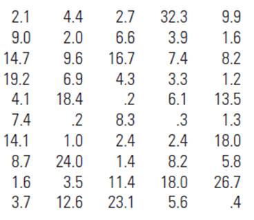
The data shows the lengths of time between the onset of a particular illness and its recurrence were recorded.

  

Calculation:

Given: the given intervals are $\overline{x}\pm s,\overline{x}\pm 2s,\text{and}\overline{x}\pm 3s$ .

Arrange the data values from smallest to largest.

  $\begin{array}{l}0.2,0.2,0.3,0.4,1,1.2,1.3,1.4,1.6,1.6,2,2.1,2.4,2.4,2.7,3.3,3.5,3.7,\\ 3.9,4.1,4.3,4.4,5.6,5.8,6.1,6.6,6.9,7.4,7.4,8.2,8.2,8.3,8.7,9,9.6,9.9,\\ 11.4,12.6,13.5,14.1,14.7,16.7,18,18,18.4,19.2,23.1,24,26.7,32.3\end{array}$

  $\text{Mean}=\frac{\text{sum}\text{of}\text{all}\text{values}}{\text{total}\text{number}\text{of}\text{values}}$

  $\begin{array}{l}\overline{x}=\frac{{\displaystyle \sum _{i=1}^n{x}_i}}{n}\\ =\frac{\begin{array}{l}0.2+0.2+0.3+0.4+1+1.2+1.3+1.4+1.6+1.6+2+2.1+2.4+2.4+2.7+3.3+3.5+3.7+\\ 3.9+4.1+4.3+4.4+5.6+5.8+6.1+6.6+6.9+7.4+7.4+8.2+8.2+8.3+8.7+9+9.6+9.9+\\ 11.4+12.6+13.5+14.1+14.7+16.7+18+18+18.4+19.2+23.1+24+26.7+32.3\end{array}}{\text{50}}\\ =\frac{418.4}{50}\\ \approx 8.37\end{array}$ find the sample variance $s^2=\frac{{\displaystyle \sum x_i{}^2-\frac{{\left({\displaystyle \sum x_i}\right)}^2}{n}}}{n-1}$

  $n=$ total number of data values.

  $n=25$

  $\begin{array}{l}{\displaystyle \sum x_i}=0.2+0.2+0.3+0.4+1+1.2+1.3+1.4+1.6+1.6+2+2.1+2.4+2.4+2.7+3.3+3.5+3.7+\\ 3.9+4.1+4.3+4.4+5.6+5.8+6.1+6.6+6.9+7.4+7.4+8.2+8.2+8.3+8.7+9+9.6+9.9+\\ 11.4+12.6+13.5+14.1+14.7+16.7+18+18+18.4+19.2+23.1+24+26.7+32.3=418.4\\ {\displaystyle \sum x_i{}^2}={0.2}^2+{0.2}^2+{0.3}^2+{0.4}^2+1^2+{1.2}^2+{1.3}^2+{1.4}^2+{1.6}^2+{1.6}^2+2^2+{2.1}^2+{2.4}^2+{2.4}^2+{2.7}^2+{3.3}^2+{3.5}^2+{3.7}^2+\\ {3.9}^2+{4.1}^2+{4.3}^2+{4.4}^2+{5.6}^2+{5.8}^2+{6.1}^2+{6.6}^2+{6.9}^2+{7.4}^2+{7.4}^2+{8.2}^2+{8.2}^2+{8.3}^2+{8.7}^2+9^2+{9.6}^2+{9.9}^2+\\ {11.4}^2+{12.6}^2+{13.5}^2+{14.1}^2+{14.7}^2+{16.7}^2+{18}^2+{18}^2+{18.4}^2+{19.2}^2+{23.1}^2+{24}^2+{26.7}^2+{32.3}^2=6384.34\end{array}$

  $\begin{array}{l}{s}^2=\frac{6384.34-\frac{{418.4}^2}{50}}{50-1}\\ =\frac{6384.34-\frac{{418.4}^2}{50}}{49}\\ \approx 58.8\end{array}$

  $s=\sqrt{58.8}=7.67$

Calculate $\overline{x}\pm s,\overline{x}\pm 2s,\text{and}\overline{x}\pm 3s$ .

  $\begin{array}{l}\overline{x}-3s=8.37-3\left(7.67\right)=-14.6\\ \overline{x}-2s=8.37-2\left(7.67\right)=-6.97\\ \overline{x}-s=8.37-7.67=0.697\\ \overline{x}+3s=8.37+3\left(7.67\right)=31.38\\ \overline{x}+2s=8.37+2\left(7.67\right)=23.7\\ \overline{x}+s=8.37+7.67=16.04\end{array}$

  $41$ of the $50$ data values lie in between $0.697$ and $16.04$ .

percentage $=\frac{41}{50}=0.82=82\%$

  $47$ of the $50$ data values lie in between $-6.97$ and $23.7$ .

percentage $=\frac{47}{50}=0.94=94\%$

  $49$ of the $50$ data values lie in between $-14.6$ and $31.38$ .

percentage $=\frac{49}{50}=0.98=98\%$

Tchebysheffs theorem states that

the observation are within one standard deviation of the mean $=$ none

the observation are within two standard deviation of the mean $=75\%$

the observation are within three standard deviation of the mean $=89\%$

The percentages agree with the Tchebysheffs theorem are $0\%,75\%\text{and}89\%$ but percentages $82\%,94\%\text{and}98\%$ are much higher than the given percentages.

Empirical theorem states that

the observation are within one standard deviation of the mean $\approx 68\%$

the observation are within two standard deviation of the mean $\approx 95\%$

the observation are within three standard deviation of the mean $\approx 99.7\%$

The percentages $82\%$ is much higher than the $68\%$ .

Hence the percentages do not agree with the Empirical rule.

c.

To determine

Explain about the Empirical rule for the given data.

Answer to Problem 2.58SE

The Empirical rule unsuitable for the given data.

Explanation of Solution

Given:

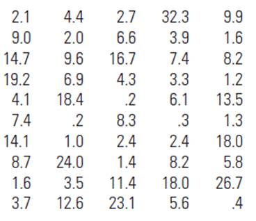
The data shows the lengths of time between the onset of a particular illness and its recurrence were recorded.

  

Calculation:

The Empirical rule only useful for mound-shaped distribution. But the given data does not have a mound-shape distribution.

Hence the Empirical rule unsuitable for the given data.