Concept explainers
Videos
Simulate five sample trajectories of Eq.
Hint: For the
Equation
where
The five sample trajectories of the equation
Answer to Problem 1P
Solution:
The five sample trajectories for
The five sample trajectories for
For
Explanation of Solution
Given information:
The discrete model for change in the price of a stock over a time interval
The parameter values are
Highly volatile have a large value for
A sequence of numbers
Explanation:
The discrete model for change in the price of a stock over a time interval
Where
The parameter values are
Substitute the above values in the equation (1)
Here,
Thus, equation (1) becomes,
Now, to find the value of
By using the computer technology,
For
Substitute the values in equation (2)
For
Substitute the values in equation (2)
For
Substitute the values in equation (2)
For
Substitute the values in equation (2)
For
Substitute the values in equation (2)
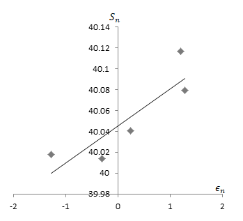
Hence, the graph of trajectories for
Now, for the value
Here,
Thus, equation (1) becomes,
Now, to find the value of
By using computer technology,
For
Substitute the values in equation (3)
For
Substitute the values in equation (3)
For
Substitute the values in equation (3)
For
Substitute the values in equation (2)
For
Substitute the values in equation (3)
The graph of trajectories for
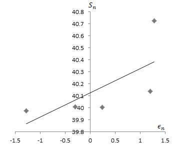
Since the approximation in the graph of trajectories for
Therefore, for
Want to see more full solutions like this?
Chapter 2 Solutions
Differential Equations: An Introduction to Modern Methods and Applications
Additional Math Textbook Solutions
Probability and Statistics for Engineers and Scientists
Thinking Mathematically (7th Edition)
Fundamentals of Differential Equations and Boundary Value Problems
A Survey of Mathematics with Applications (10th Edition) - Standalone book
Calculus for Business, Economics, Life Sciences, and Social Sciences (13th Edition)
Finite Mathematics for Business, Economics, Life Sciences and Social Sciences


- For the regression model Yi = b0 + eI, derive the least squares estimator.arrow_forward1)A new starch polymer foam with high shock absorbent properties is expected to perform better thanthe old foam which can withstand a maximum impact of 1.56 Joule (J). A simple destructive testto quantify shock absorption ability of the new foam is conducted. Table 5 shows the impact energyabsorbed (in J) that the new foam can withstand for each test. Table 51.61 1.5 1.65 1.7 1.4 1.59 1.65 1.5 Does the recorded data suggests that the new foam performs better than the old foam? Use 2.5%level of significance. 2) A number of 28 university students who smokes completed a questionnaire inquiring their smokinghistory and behavior. The result shows that the average smoking initiation age of this group is 21.6years with a variance of 18.49. Based on past record, the smoking initiation age of universitystudent has a mean of 20.74 years with a standard deviation of 5.1 years. Conduct a necessaryanalysis to determine if the smoking initiation age remain the same as the previous record.…arrow_forwardGiven the residuals squared derived from the regression: Marks = ƒ(Study hours) Use the information from the following auxiliary regression (table attached) to conduct the Park test to detect for the presence of heteroscedasticity at a = 5%.arrow_forward
- The accompanying dataset provides data on the monthly usage of natural gas (in millions of cubic feet) for a certain region over two years. Implement the Holt-Winters multiplicative seasonality model with no trend to find the forecast for periods 13-26, where alphaαequals=0.50.5 and gammaγequals=0.80.8. Then find the MAD for periods 13-24. Month Period Gas Usage Jan 1 242 Feb 2 227 Mar 3 153 Apr 4 144 May 5 55 Jun 6 34 Jul 7 29 Aug 8 27 Sep 9 28 Oct 10 40 Nov 11 88 Dec 12 203 Jan 13 231 Feb 14 248 Mar 15 251 Apr 16 139 May 17 35 Jun 18 32 Jul 19 28 Aug 20 26 Sep 21 27 Oct 22 38 Nov 23 86 Dec 24 182 Use the Holt-Winters multiplicative seasonality model with no trend to find the forecast for periods 13-18, periods 19-24, and then for periods 25 and 26. (Type integers or decimals rounded to two decimal places as needed.) Period Forecast 13 14 15 16 17 18arrow_forwardWhen the classical linear model assumptions are fulfilled, the OLS estimator is... t-distributed with n-k-1 degrees of freedom. Constant. Normally distributed. F distributed.arrow_forwardThe below time series gives the indices of Industrial Production in U.S for 10 consecutive years. Year IP 1 79.62 2 86.54 3 88.14 4 89.23 5 93.45 6 97.4 7 99.34 8 96.98 9 100.22 10 103.56 Construct a time series plot. What type of pattern exists in the data? Use simple linear regression analysis to find the parameters for the line that minimizes MSE for this time series. What is the forecast for t = 11?arrow_forward
- Suppose your dependent variable is aggregate household demand for electricity for various cities. To correct for heteroskedasticity you should Select one: a. multiply observations by the square root of the city size b. multiply observations by the city size c. divide observations by the city size d. divide observations by the square root of the city size e. none of thesearrow_forwardConsider the following datasets: X1=2,8,4 X2= 0.4, 7.10, 3.2 Y= 2.6, 9.2, 5.3 Statistically regress Y on X1 and X2, i.e. find a regression equation in which output variable is Y and input variable is X1 and X2. Show first two iterations of Gradient Descent method to solve part a. Initialize slopes and intercept at 0 value.arrow_forwardThe following partial JMP regression output for the Fresh detergent data relates to predicting demand for future sales periods in which the price difference will be .10. SE Fit = .165360573, s = .628152. Predicted Demand Lower 95% MeanDemand Upper 95% MeanDemand 31 8.181072245 7.842346262 8.519798229 StdErr IndivDemand Lower 95% IndivDemand Upper 95% MeanDemand 0.649552965 6.850522511 9.511621980 Click here for the Excel Data File (a) Report a point estimate of and a 95 percent confidence interval for the mean demand for Fresh in all sales periods when the price difference is .10. (Round your CI answers to 3 decimal places and other answer to 4 decimal places.) (b) Report a point prediction of and a 95 percent prediction interval for the actual demand for Fresh in an individual sales period when the price difference is .10. (Round your PI answers to 3 decimal places and other answer to 4 decimal places.) (c) StdErr Indiv Demand on…arrow_forward
- The following estimated regression model was developed relating yearly income (y in $1000s) of 30 individuals with their age (x1) and their gender (x2) (0 if male and 1 if female).ŷ = 30 + 0.7x1 + 3x2Also provided are SST = 1200 and SSE = 384.The yearly income of a 24-year-old female individual is _____.arrow_forward5 How does the dynamic CCE estimator solve the estimation problems of the PMG technique?arrow_forwardUse a smoothing constant ALPHA = 0.8 and calculate the forecasted value and smoothing valuearrow_forward
 Linear Algebra: A Modern IntroductionAlgebraISBN:9781285463247Author:David PoolePublisher:Cengage Learning
 Glencoe Algebra 1, Student Edition, 9780079039897...AlgebraISBN:9780079039897Author:CarterPublisher:McGraw Hill