
Concept explainers
Videos
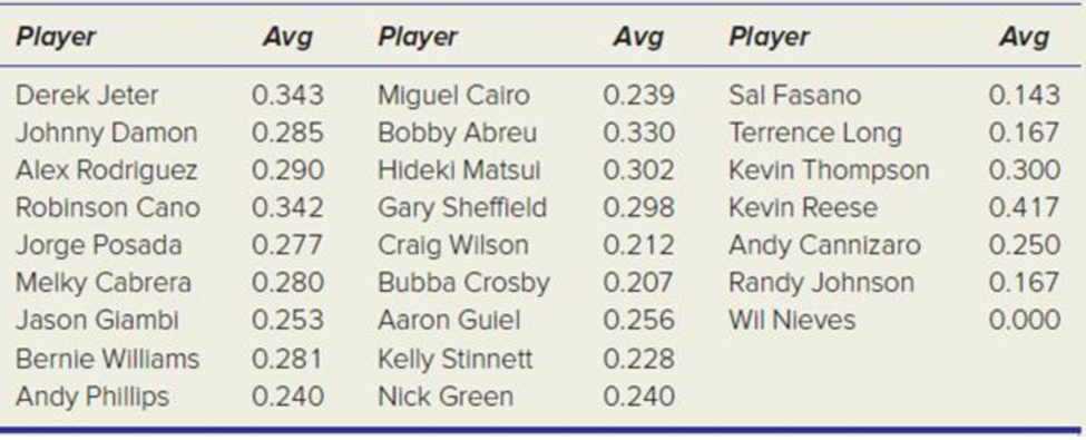
Below are batting averages of the New York Yankees players who were at bat five times or more in 2006. (a) Construct a frequency distribution. Explain how you chose the number of bins and the bin limits. (b) Make a histogram and describe its appearance. (c) Repeat, using a different number of bins and different bin limits. (d) Did your visual impression of the data change when you changed the number of bins? Explain.
Batting Averages for the 2006 New York Yankees
a.
Construct a frequency distribution and explain how the number of bins and the bin limits are chosen.
Answer to Problem 30CE
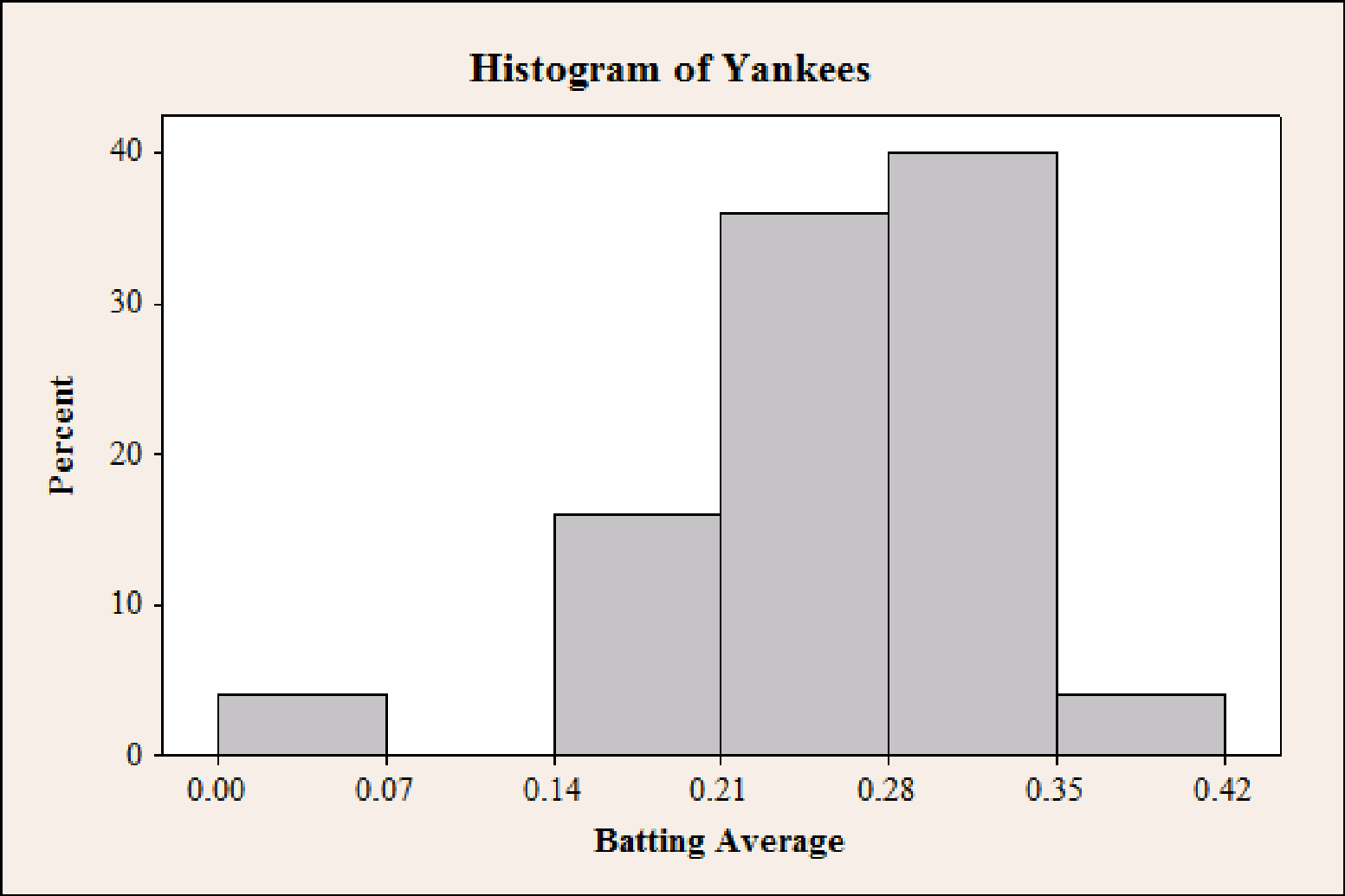
Thefrequency distribution is tabulated below,
| Bin limits | Mid point | Width |
Frequency | Percent | Cumulative | ||
| Lower | Upper | Frequency | Percent | ||||
| 0 | < 0.07 | 0.035 | 0.07 | 1 | 4 | 1 | 4 |
| 0.07 | < 0.14 | 0.105 | 0.07 | 0 | 0 | 1 | 4 |
| 0.14 | < 0.21 | 0.175 | 0.07 | 4 | 16 | 5 | 20 |
| 0.21 | < 0.28 | 0.245 | 0.07 | 9 | 36 | 14 | 56 |
| 0.28 | < 0.35 | 0.315 | 0.07 | 10 | 40 | 24 | 96 |
| 0.35 | < 0.42 | 0.385 | 0.07 | 1 | 4 | 25 | 100 |
| Total | |||||||
Explanation of Solution
Calculation:
The given information is that, the data representsthebatting averages of the New York Yankees players who were at bat five times or more in 2006.
Frequency distribution:
It is a tabulation of n data values which are divided into k classes called bins. The bin limits are the cutoff points which defines each bin. These generally have equal interval and the limits do not overlap.
Step-by-step procedure to construct frequency distribution table is as follows:
- • The smallest and largest data values are 0 and 0.417.
- • Here the sample size is 25. By Sturge’s Rule,
- • Bin width is obtained by dividing the range by the number of bins.
Hence, the bin width is 0.07.
- • The minimum value in the data is 0 hence the first bin should start at 0.
Tally mark:
- • Make a tally mark for each score in the corresponding class and continue for all reading times in the data.
- • The number of tally marks in each class represents the frequency, f of that class.
Thus, the frequency distribution table is as follows:
| Bin limits | Tally |
Frequency | Percent | |
| Lower | Upper | |||
| 0 | < 0.07 | 1 | ||
| 0.07 | < 0.14 | 0 | ||
| 0.14 | < 0.21 | 4 | ||
| 0.21 | < 0.28 | 9 | ||
| 0.28 | < 0.35 | 10 | ||
| 0.35 | < 0.42 | 1 | ||
| Total | 25 | |||
Mid point:
The midpoint is the average of the lower limit and upper limit of a particular class. It is also called as class mark.
Thus, the mid points for each class is tabulated below:
| Bin limits |
Frequency | Mid point | |
| Lower | Upper | ||
| 0 | < 0.07 | 1 | |
| 0.07 | < 0.14 | 0 | |
| 0.14 | < 0.21 | 4 | |
| 0.21 | < 0.28 | 9 | |
| 0.28 | < 0.35 | 10 | |
| 0.35 | < 0.42 | 1 | |
| Total | 25 | ||
Cumulative frequency:
Cumulative frequency is the sum of all frequencies up to that class. The last class’s cumulative frequency is equal to the sample size
Thus, the cumulative frequency for each calss is tabulated below:
| Bin limits |
Frequency |
Cumulative frequency | |
| Lower | Upper | ||
| 0 | < 0.07 | 1 | 1 |
| 0.07 | < 0.14 | 0 | |
| 0.14 | < 0.21 | 4 | |
| 0.21 | < 0.28 | 9 | |
| 0.28 | < 0.35 | 10 | |
| 0.35 | < 0.42 | 1 | |
| Total | 25 | ||
Cumulative Relative frequency:
| Bin limits |
Cumulative frequency |
Cumulative percent | |
| Lower | Upper | ||
| 0 | < 0.07 | 1 | |
| 0.07 | < 0.14 | 1 | |
| 0.14 | < 0.21 | 5 | |
| 0.21 | < 0.28 | 14 | |
| 0.28 | < 0.35 | 24 | |
| 0.35 | < 0.42 | 25 | |
| Total | |||
b.
Constuct a histogram and describe its appearance.
Answer to Problem 30CE
The histogram for the data is as follows,
Explanation of Solution
Calculation:
Software procedure:
Step-by-step procedure to obtain histogram using MINITAB software is as follows,
- • Choose Graph > Histogram.
- • Choose Simple, and then click OK.
- • In Graph variables, enter the corresponding column of Yankees.
- • Click Scale>Y-Scale Type > Percent
- • Click OK.
- • To modify the interval settings, double click on the horizontal axis of the graph. Then, select Binning>Cutpoint>Cutpoint Positions, in this box, enter the values for the cut points of the bin intervals (0, 0.07, 0.14, 0.21, 0.28, 0.35 and 0.42).
From the histogram it is observed that the tail on the left is more elongated than the tail on the right. Hence the distribution of the histogram seems to be skewed left.
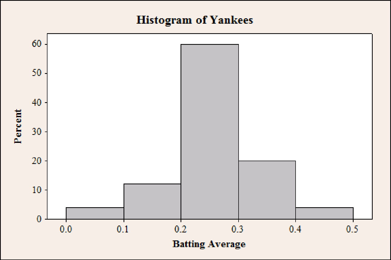
c.
Repeat the procedure using different number of bins and different bin limits.
Answer to Problem 30CE
Thefrequency distribution using 5 bins is as follows,
| Bin limits | Mid point | Width |
Frequency | Percent | Cumulative | ||
| Lower | Upper | Frequency | Percent | ||||
| 0 | < 0.1 | 0.05 | 0.1 | 1 | 4 | 1 | 4 |
| 0.1 | < 0.2 | 0.15 | 0.1 | 3 | 12 | 4 | 16 |
| 0.2 | < 0.3 | 0.25 | 0.1 | 15 | 60 | 19 | 76 |
| 0.3 | < 0.4 | 0.35 | 0.1 | 5 | 20 | 24 | 96 |
| 0.4 | < 0.5 | 0.45 | 0.1 | 1 | 4 | 25 | 100 |
| Total | |||||||
The histogram for 5 bins with 0.1 width is as follows,
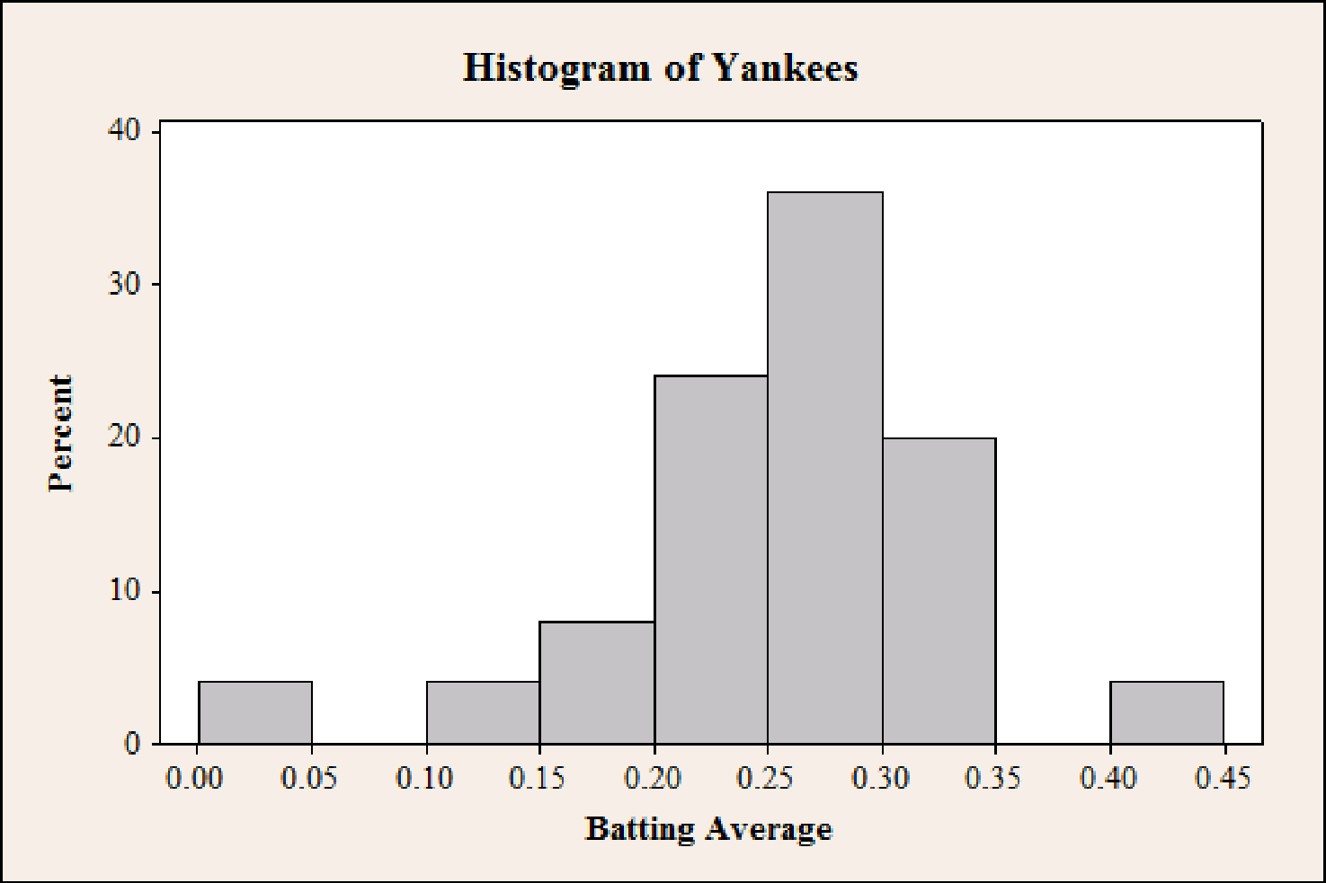
Thefrequency distribution using 0.15 width and 9 bins is as follows,
| Bin limits | Mid point | Width |
Frequency | Percent | Cumulative | ||
| Lower | Upper | Frequency | Percent | ||||
| 0 | < 0.05 | 0.025 | 0.05 | 1 | 4 | 1 | 4 |
| 0.05 | < 0.10 | 0.075 | 0.05 | 0 | 0 | 1 | 4 |
| 0.10 | < 0.15 | 0.125 | 0.05 | 1 | 4 | 2 | 8 |
| 0.15 | < 0.20 | 0.175 | 0.05 | 2 | 8 | 4 | 16 |
| 0.20 | < 0.25 | 0.225 | 0.05 | 6 | 24 | 10 | 40 |
| 0.25 | < 0.30 | 0.275 | 0.05 | 9 | 36 | 19 | 76 |
| 0.30 | < 0.35 | 0.325 | 0.05 | 5 | 20 | 24 | 96 |
| 0.35 | < 0.40 | 0.375 | 0.05 | 0 | 0 | 24 | 96 |
| 0.45 | < 0.45 | 0.425 | 0.05 | 1 | 4 | 25 | 100 |
| Total | |||||||
The histogram for 9 bins with width 0.05 is as follows,
Explanation of Solution
Calculation:
For 5 bins:
Here the number of bins are considered as 5 with width 0.1.
| Bin limits | Tally |
Frequency | Percent | |
| Lower | Upper | |||
| 0 | < 0.1 | 1 | ||
| 0.1 | < 0.2 | 3 | ||
| 0.2 | < 0.3 | 15 | ||
| 0.3 | < 0.4 | 5 | ||
| 0.4 | < 0.5 | 1 | ||
| Total | 25 | |||
Mid point:
The midpoint is the average of the lower limit and upper limit of a particular class. It is also called as class mark.
Thus, the mid points for each class is tabulated below:
| Bin limits |
Frequency | Mid point | |
| Lower | Upper | ||
| 0 | < 0.1 | 1 | |
| 0.1 | < 0.2 | 3 | |
| 0.2 | < 0.3 | 15 | |
| 0.3 | < 0.4 | 5 | |
| 0.4 | < 0.5 | 1 | |
| Total | 25 | ||
Cumulative frequency:
Cumulative frequency is the sum of all frequencies up to that class. The last class’s cumulative frequency is equal to the sample size
Thus, the cumulative frequency for each calss is tabulated below:
| Bin limits |
Frequency |
Cumulative frequency | |
| Lower | Upper | ||
| 0 | < 0.1 | 1 | 1 |
| 0.1 | < 0.2 | 3 | |
| 0.2 | < 0.3 | 15 | |
| 0.3 | < 0.4 | 5 | |
| 0.4 | < 0.5 | 1 | |
| Total | 25 | ||
Cumulative Relative frequency:
| Bin limits |
Cumulative frequency |
Cumulative percent | |
| Lower | Upper | ||
| 0 | < 0.1 | 1 | |
| 0.1 | < 0.2 | 4 | |
| 0.2 | < 0.3 | 19 | |
| 0.3 | < 0.4 | 24 | |
| 0.4 | < 0.5 | 25 | |
| Total | |||
Software procedure:
Step-by-step software procedure to obtain histogram using MINITAB software is as follows,
- • Choose Graph > Histogram.
- • Choose Simple, and then click OK.
- • In Graph variables, enter the corresponding column of Yankees.
- • Click Scale>Y-Scale Type> Percent
- • Click OK.
- • To modify the interval settings, double click on the horizontal axis of the graph. Then, select Binning>Cutpoint>CutpointPositions,in this box, enter the values for the cut points of the bin intervals (0, 0.1, 0.2, 0.3, 0.4 and 0.5).
- For 9 bins:
Here the number of bins are considered as 9 with width 0.05.
The frequeny table is as follows,
| Bin limits | Tally |
Frequency | Percent | |
| Lower | Upper | |||
| 0 | < 0.05 | 1 | ||
| 0.05 | < 0.10 | 0 | ||
| 0.10 | < 0.15 | 1 | ||
| 0.15 | < 0.20 | 2 | ||
| 0.20 | < 0.25 | 6 | ||
| 0.25 | < 0.30 | 9 | ||
| 0.30 | < 0.35 | 5 | ||
| 0.35 | < 0.40 | 0 | ||
| 0.45 | < 0.45 | 1 | ||
| Total | 25 | |||
Mid point:
The midpoint is the average of the lower limit and upper limit of a particular class. It is also called as class mark.
Thus, the mid points for each class is tabulated below:
| Bin limits |
Frequency | Mid point | |
| Lower | Upper | ||
| 0 | < 0.05 | 1 | |
| 0.05 | < 0.10 | 0 | |
| 0.10 | < 0.15 | 1 | |
| 0.15 | < 0.20 | 2 | |
| 0.20 | < 0.25 | 6 | |
| 0.25 | < 0.30 | 9 | |
| 0.30 | < 0.35 | 5 | |
| 0.35 | < 0.40 | 0 | |
| 0.40 | < 0.45 | 1 | |
| Total | 25 | ||
Cumulative frequency:
Cumulative frequency is the sum of all frequencies up to that class. The last class’s cumulative frequency is equal to the sample size
Thus, the cumulative frequency for each calss is tabulated below:
| Bin limits |
Frequency |
Cumulative frequency | |
| Lower | Upper | ||
| 0 | < 0.05 | 1 | 1 |
| 0.05 | < 0.10 | 0 | |
| 0.10 | < 0.15 | 1 | |
| 0.15 | < 0.20 | 2 | |
| 0.20 | < 0.25 | 6 | |
| 0.25 | < 0.30 | 9 | |
| 0.30 | < 0.35 | 5 | |
| 0.35 | < 0.40 | 0 | |
| 0.40 | < 0.45 | 1 | |
| Total | 25 | ||
Cumulative Relative frequency:
| Bin limits |
Cumulative frequency |
Cumulative percent | |
| Lower | Upper | ||
| 0 | < 0.05 | 1 | |
| 0.05 | < 0.10 | 1 | |
| 0.10 | < 0.15 | 2 | |
| 0.15 | < 0.20 | 4 | |
| 0.20 | < 0.25 | 10 | |
| 0.25 | < 0.30 | 19 | |
| 0.30 | < 0.35 | 24 | |
| 0.35 | < 0.40 | 24 | |
| 0.40 | < 0.45 | 25 | |
| Total | |||
Software procedure:
Step-by-step software procedure to obtain histogram using MINITAB software is as follows,
- • Choose Graph > Histogram.
- • Choose Simple, and then click OK.
- • In Graph variables, enter the corresponding column of Yankees.
- • Click Scale>Y-Scale Type> Percent
- • Click OK.
- • To modify the interval settings, double click on the horizontal axis of the graph. Then, select Binning>Cutpoint>CutpointPositions,in this box, enter the values for the cut points of the bin intervals (0, 0.05, 0.10, 0.15, 0.20, 0.25, 0.30, 0.35, 0.40 and 0.45).
d.
Explain whether the visual impression of the data change when the number of bins increased or not
Answer to Problem 30CE
Yes, the visual impression of the data changes when the number of bins are varied.
Explanation of Solution
From the histograms in part (c), it is observed that when the bins are 5 the histogram appears to be more symmetrical. And when the bins are 9 then, the histogram appears to be skewed left. Hence there is change the appearance of the histogram when the number of bins vary.
Want to see more full solutions like this?
Chapter 3 Solutions
Applied Statistics in Business and Economics


 Glencoe Algebra 1, Student Edition, 9780079039897...AlgebraISBN:9780079039897Author:CarterPublisher:McGraw Hill
 Big Ideas Math A Bridge To Success Algebra 1: Stu...AlgebraISBN:9781680331141Author:HOUGHTON MIFFLIN HARCOURTPublisher:Houghton Mifflin Harcourt
 Holt Mcdougal Larson Pre-algebra: Student Edition...AlgebraISBN:9780547587776Author:HOLT MCDOUGALPublisher:HOLT MCDOUGAL