Table 3.P.1 lists drug concentration measurements made in blood and tissue compartments over a period of
100
min. Use the method described in problems 2 through 4 to estimate the rate coefficients
k
01
,
k
12
and
k
21
in the system model (1). Then solve the resulting system using initial conditions from line 1 of Table 3.P.1. Verify the accuracy of your estimates by plotting the solution components and the data in Table 3.P.1 on the same set of coordinate axes.
TABLE 3.P.1 Compartment concentration measurements.
time
(min)
x
1
(
mg/mL
)
x
2
(
mg/mL
)
0.000
0.623
0.000
7.143
0.374
0.113
14.286
0.249
0.151
21.429
0.183
0.157
28.571
0.145
0.150
35.714
0.120
0.137
42.857
0.103
0.124
50.000
0.089
0.110
57.143
0.078
0.098
64.286
0.068
0.087
71.429
0.060
0.077
78.571
0.053
0.068
85.714
0.047
0.060
92.857
0.041
0.053
100.000
0.037
0.047
Estimating Eigenvalues and Eigenvectors of
K
from Transient Concentration Data. Denote by
x
*
(
t
k
)
=
x
1
*
(
t
k
)
i
+
x
2
*
(
t
k
)
j
,
k
=
1
,
2
,
3
,
…
measurements of the concentrations in each of the compartments. We assume that the eigenvalues of
K
satisfy
λ
2
<
λ
1
<
0
. Denote the eigenvectors of
λ
1
and
λ
2
by
V
1
=
(
v
11
v
21
)
and
V
2
=
(
v
12
v
22
)
,
respectively. The solution of Eq. (1) can be expressed as
X
(
t
)
=
α
e
λ
1
t
v
1
+
β
e
λ
2
t
v
2
, (i)
where
α
and
β
, assumed to be nonzero, depend on initial conditions. From Eq. (i), we note that
x
(
t
)
=
e
λ
1
t
[
α
v
1
+
β
e
(
λ
2
−
λ
1
)
t
v
2
]
~
α
e
λ
1
t
v
1
if
e
(
λ
2
−
λ
1
)
t
~
0
.
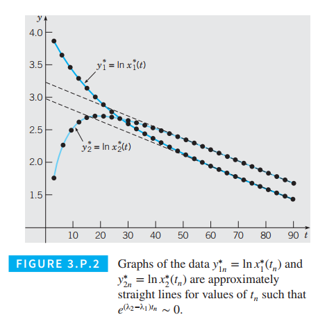
(a) For values of
t
such that
e
(
λ
2
−
λ
1
)
t
~
0
, explain why the graphs of
ln
x
1
(
t
)
and
ln
x
2
(
t
)
should be approximately straight lines with slopes equal to
λ
1
and intercepts equal to
ln
α
v
11
and
ln
α
v
21
, respectively. Thus estimates of
λ
1
,
α
v
11
, and
α
v
21
may be obtained by fitting straight lines to the data
ln
x
1
*
(
t
n
)
and
ln
x
2
*
(
t
n
)
corresponding to values of
t
n
, where graphs of the logarithms of the data are approximately linear, as shown in Figure 3.P.2.
Given that both components of the data
x
*
(
t
n
)
are accurately represented by a sum of exponential functions of the form (i), explain how to find estimates of
λ
2
,
β
v
12
, and
β
v
22
using the residual data
x
r
*
(
t
n
)
=
x
*
(
t
n
)
−
v
^
(
α
)
e
λ
1
t
n
, where estimates of
λ
1
and
α
v
1
are denoted by
λ
^
1
and
v
^
(
α
)
, respectively.
Computing the Entries of
K
from Its Eigenvalues and Eigenvectors. Assume that the eigenvalues
λ
1
and
λ
2
and corresponding eigenvectors
v
1
and
v
2
of
K
are known. Show that the entries of the matrix
K
must satisfy the following systems of equations:
(
v
11
v
21
v
12
v
22
)
(
k
11
k
12
)
=
(
λ
1
v
11
λ
2
v
12
)
(iii)
and
(
v
11
v
21
v
12
v
22
)
(
k
21
k
22
)
=
(
λ
1
v
21
λ
2
v
22
)
(iv)
or, using matrix notation,
K
V
=
V
Λ
, where
V
=
(
v
11
v
21
v
12
v
22
)
and
Λ
=
(
λ
1
0
0
λ
2
)
Given estimates
K
^
i
j
of the entries of
K
and estimates
λ
^
1
and
λ
^
2
of the eigenvalues of
K
, show how to obtain an estimate
K
^
01
of
K
01
using the relations in Problem 1(b).


 Linear Algebra: A Modern IntroductionAlgebraISBN:9781285463247Author:David PoolePublisher:Cengage Learning