Concept explainers
Videos
If we are going to use data from this year to predict unemployment next year’s unemployment? A model like this, in which previous values of a variable are used to predict future values of the same variables. Is called an autoregressive model. The following table presents the needed to fit this model.
Compute the least-square line for predicting next year’s unemployment from this year’s unemployment.
To calculate:
To compute the least squares regression line for predicting next year’s unemployment from this year’s unemployment.
Answer to Problem 10CS
Explanation of Solution
Given information:
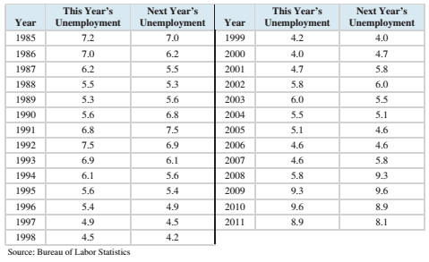
A model in which previous values of a variable are used to predict future values of the same variable is called an autoregressive model. The following table presents the data needed to fit this model.
| Year | This Year’sUnemployment | Next Year’sUnemployment |
| 1985 | 7.2 | 7.0 |
| 1986 | 7.0 | 6.2 |
| 1987 | 6.2 | 5.5 |
| 1988 | 5.5 | 5.3 |
| 1989 | 5.3 | 5.6 |
| 1990 | 5.6 | 6.8 |
| 1991 | 6.8 | 7.5 |
| 1992 | 7.5 | 6.9 |
| 1993 | 6.9 | 6.1 |
| 1994 | 6.1 | 5.6 |
| 1995 | 5.6 | 5.4 |
| 1996 | 5.4 | 4.9 |
| 1997 | 4.9 | 4.5 |
| 1998 | 4.5 | 4.2 |
| 1999 | 4.2 | 4.0 |
| 2000 | 4.0 | 4.7 |
| 2001 | 4.7 | 5.8 |
| 2002 | 5.8 | 6.0 |
| 2003 | 6.0 | 5.5 |
| 2004 | 5.5 | 5.1 |
| 2005 | 5.1 | 4.6 |
| 2006 | 4.6 | 4.6 |
| 2007 | 4.6 | 5.8 |
| 2008 | 5.8 | 9.3 |
| 2009 | 9.3 | 9.6 |
| 2010 | 9.6 | 8.9 |
| 2011 | 8.9 | 8.1 |
Formula Used:
The equation for least-square regression line:
Where
The correlation coefficient of a data is given by:
Where,
The standard deviations are given by:
The mean of x is given by:
The mean of y is given by:
Calculation:
The mean of x is given by:
The mean of y is given by:
The data can be represented in tabular form as:
| x | y |  |
 |
 |
 |
| 7.2 | 7.0 | 1.17778 | 1.38716 | 0.94444 | 0.89198 |
| 7.0 | 6.2 | 4.12963 | 17.05384 | 0.14444 | 0.02086 |
| 6.2 | 5.5 | 3.32963 | 11.08643 | -0.55556 | 0.30864 |
| 5.5 | 5.3 | 2.62963 | 6.91495 | -0.75556 | 0.57086 |
| 5.3 | 5.6 | 2.42963 | 5.90310 | -0.45556 | 0.20753 |
| 5.6 | 6.8 | 2.72963 | 7.45088 | 0.74444 | 0.55420 |
| 6.8 | 7.5 | 3.92963 | 15.44199 | 1.44444 | 2.08642 |
| 7.5 | 6.9 | 4.62963 | 21.43347 | 0.84444 | 0.71309 |
| 6.9 | 6.1 | 4.02963 | 16.23791 | 0.04444 | 0.00198 |
| 6.1 | 5.6 | 3.22963 | 10.43051 | -0.45556 | 0.20753 |
| 5.6 | 5.4 | 2.72963 | 7.45088 | -0.65556 | 0.42975 |
| 5.4 | 4.9 | 2.52963 | 6.39903 | -1.15556 | 1.33531 |
| 4.9 | 4.5 | 2.02963 | 4.11940 | -1.55556 | 2.41975 |
| 4.5 | 4.2 | 1.62963 | 2.65569 | -1.85556 | 3.44309 |
| 4.2 | 4.0 | 1.32963 | 1.76791 | -2.05556 | 4.22531 |
| 4.0 | 4.7 | 1.12963 | 1.27606 | -1.35556 | 1.83753 |
| 4.7 | 5.8 | 1.82963 | 3.34754 | -0.25556 | 0.06531 |
| 5.8 | 6.0 | 2.92963 | 8.58273 | -0.05556 | 0.00309 |
| 6.0 | 5.5 | 3.12963 | 9.79458 | -0.55556 | 0.30864 |
| 5.5 | 5.1 | 2.62963 | 6.91495 | -0.95556 | 0.91309 |
| 5.1 | 4.6 | 2.22963 | 4.97125 | -1.45556 | 2.11864 |
| 4.6 | 4.6 | 1.72963 | 2.99162 | -1.45556 | 2.11864 |
| 4.6 | 5.8 | 1.72963 | 2.99162 | -0.25556 | 0.06531 |
| 5.8 | 9.3 | 2.92963 | 8.58273 | 3.24444 | 10.52642 |
| 9.3 | 9.6 | 6.42963 | 41.34014 | 3.54444 | 12.56309 |
| 9.6 | 8.9 | 6.72963 | 45.28791 | 2.84444 | 8.09086 |
| 8.9 | 8.1 | 6.02963 | 36.35643 | 2.04444 | 4.17975 |
| |
|
|
|
Hence, the standard deviation is given by:
And,
Consider,
Hence, the table for calculating coefficient of correlation is given by:
| x | y |  |
 |
 |
| 7.2 | 7.0 | 1.17778 | 0.94444 | 1.11235 |
| 7.0 | 6.2 | 4.12963 | 0.14444 | 0.59650 |
| 6.2 | 5.5 | 3.32963 | -0.55556 | -1.84979 |
| 5.5 | 5.3 | 2.62963 | -0.75556 | -1.98683 |
| 5.3 | 5.6 | 2.42963 | -0.45556 | -1.10683 |
| 5.6 | 6.8 | 2.72963 | 0.74444 | 2.03206 |
| 6.8 | 7.5 | 3.92963 | 1.44444 | 5.67613 |
| 7.5 | 6.9 | 4.62963 | 0.84444 | 3.90947 |
| 6.9 | 6.1 | 4.02963 | 0.04444 | 0.17909 |
| 6.1 | 5.6 | 3.22963 | -0.45556 | -1.47128 |
| 5.6 | 5.4 | 2.72963 | -0.65556 | -1.78942 |
| 5.4 | 4.9 | 2.52963 | -1.15556 | -2.92313 |
| 4.9 | 4.5 | 2.02963 | -1.55556 | -3.15720 |
| 4.5 | 4.2 | 1.62963 | -1.85556 | -3.02387 |
| 4.2 | 4.0 | 1.32963 | -2.05556 | -2.73313 |
| 4.0 | 4.7 | 1.12963 | -1.35556 | -1.53128 |
| 4.7 | 5.8 | 1.82963 | -0.25556 | -0.46757 |
| 5.8 | 6.0 | 2.92963 | -0.05556 | -0.16276 |
| 6.0 | 5.5 | 3.12963 | -0.55556 | -1.73868 |
| 5.5 | 5.1 | 2.62963 | -0.95556 | -2.51276 |
| 5.1 | 4.6 | 2.22963 | -1.45556 | -3.24535 |
| 4.6 | 4.6 | 1.72963 | -1.45556 | -2.51757 |
| 4.6 | 5.8 | 1.72963 | -0.25556 | -0.44202 |
| 5.8 | 9.3 | 2.92963 | 3.24444 | 9.50502 |
| 9.3 | 9.6 | 6.42963 | 3.54444 | 22.78947 |
| 9.6 | 8.9 | 6.72963 | 2.84444 | 19.14206 |
| 8.9 | 8.1 | 6.02963 | 2.04444 | 12.32724 |
| |
|
|
Plugging the values in the formula,
Plugging the values to obtain b1,
Plugging the values to obtain b0,
Hence, the least-square regression line is given by:
Therefore, the least squares regression line for the given data set is
Want to see more full solutions like this?
Chapter 4 Solutions
ELEMENTARY STAT.(LL) >CUSTOM PACKAGE<


- Olympic Pole Vault The graph in Figure 7 indicates that in recent years the winning Olympic men’s pole vault height has fallen below the value predicted by the regression line in Example 2. This might have occurred because when the pole vault was a new event there was much room for improvement in vaulters’ performances, whereas now even the best training can produce only incremental advances. Let’s see whether concentrating on more recent results gives a better predictor of future records. (a) Use the data in Table 2 (page 176) to complete the table of winning pole vault heights shown in the margin. (Note that we are using x=0 to correspond to the year 1972, where this restricted data set begins.) (b) Find the regression line for the data in part ‚(a). (c) Plot the data and the regression line on the same axes. Does the regression line seem to provide a good model for the data? (d) What does the regression line predict as the winning pole vault height for the 2012 Olympics? Compare this predicted value to the actual 2012 winning height of 5.97 m, as described on page 177. Has this new regression line provided a better prediction than the line in Example 2?arrow_forwardRepeat Example 5 when microphone A receives the sound 4 seconds before microphone B.arrow_forward
 Linear Algebra: A Modern IntroductionAlgebraISBN:9781285463247Author:David PoolePublisher:Cengage Learning
 College AlgebraAlgebraISBN:9781305115545Author:James Stewart, Lothar Redlin, Saleem WatsonPublisher:Cengage Learning
 Trigonometry (MindTap Course List)TrigonometryISBN:9781337278461Author:Ron LarsonPublisher:Cengage Learning