
Concept explainers
(a)
The histogram frequency distribution, cumulative percentage distribution for each set of data and average speed.
Answer to Problem 10P
Explanation of Solution
Given:
Significance level of

Formula used:
Calculation:
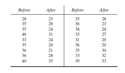
Before an increase in speed enforcement activities:
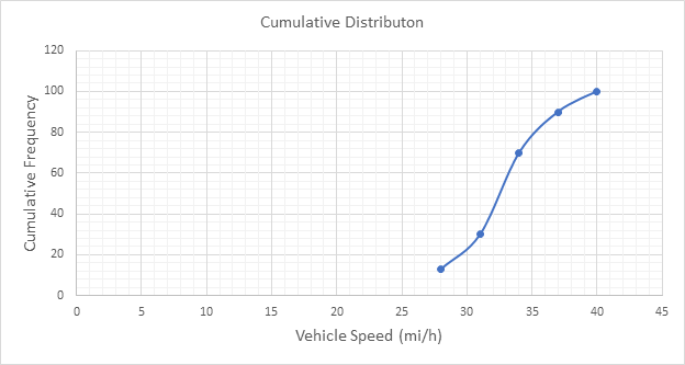
The speed ranges from 28 to 40 mi/h giving a speed range of 12. For five classes, the range per class is 2.4 mi/h. A frequency distribution table can then be prepared, as shown below in which the speed classes are listed in column 1 and the mid-values are in column 2. The number of observations for each class is listed in column 3 and the cumulative percentages of all observations are listed in column 6.
| 1 | 2 | 3 | 4 | 5 | 6 | 7 |
| Speed class (mi/h) | Class mid-value | Class frequency, | Percentage of class frequency | Cumulative percentage of class frequency | ||
| 28-30 | 29 | 4 | 116 | 13 | 13 | 139.24 |
| 31-33 | 32 | 5 | 160 | 17 | 30 | 42.05 |
| 34-36 | 35 | 12 | 420 | 40 | 70 | 0.12 |
| 37-39 | 38 | 6 | 228 | 20 | 90 | 57.66 |
| 40-42 | 41 | 3 | 123 | 10 | 100 | 111.63 |
| Total | 30 | 1047 | 350.7 |
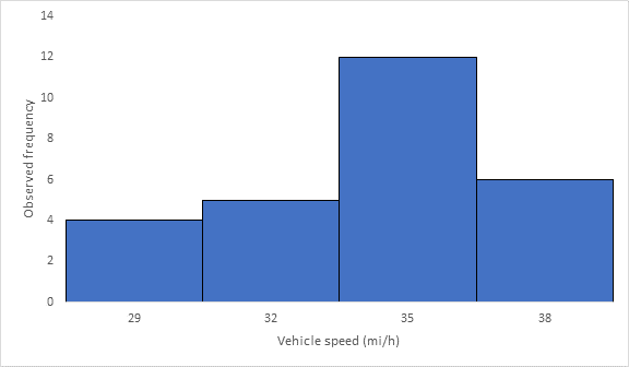
Below Figure shows the frequency histogram for the data shown in above Table. The values in columns 2 and 3 of Table are used to draw the frequency histogram, where the abscissa represents the speeds and the ordinate the observed frequency in each class.

Below Figure shows the cumulative frequency distribution curve for the data given. In this case, the cumulative percentages in column 6 of above Table are plotted against the upper limit of each corresponding speed class. This curve gives the percentage of vehicles that are traveling at or below a given speed.

Determine the arithmetic mean speed:
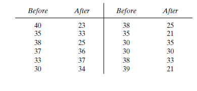
After an increase in speed enforcement activities:
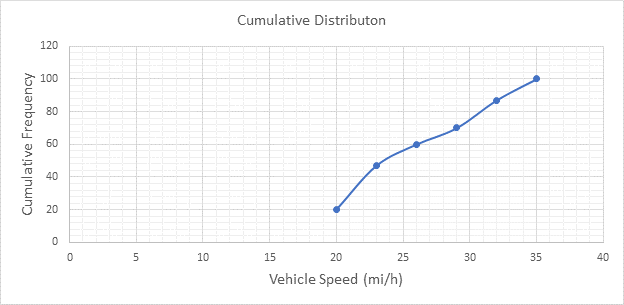
The speed ranges from 20 to 37 mi/h giving a speed range of 17. For six classes, the range per class is 2.83 mi/h. A frequency distribution table can then be prepared, as shown below in which the speed classes are listed in column 1 and the mid-values are in column 2. The number of observations for each class is listed in column 3 and the cumulative percentages of all observations are listed in column 6.
| 1 | 2 | 3 | 4 | 5 | 6 | 7 |
| Speed class (mi/h) | Class mid-value | Class frequency, | Percentage of class frequency | Cumulative percentage of class frequency | ||
| 20-22 | 21 | 6 | 126 | 20 | 20 | 253.5 |
| 23-25 | 24 | 8 | 192 | 27 | 47 | 98 |
| 26-28 | 27 | 4 | 108 | 13 | 60 | 1 |
| 29-31 | 30 | 3 | 90 | 10 | 70 | 18.75 |
| 32-34 | 33 | 5 | 165 | 17 | 87 | 151.25 |
| 35-37 | 36 | 4 | 144 | 13 | 100 | 289 |
| Total | 30 | 825 | 811.5 |
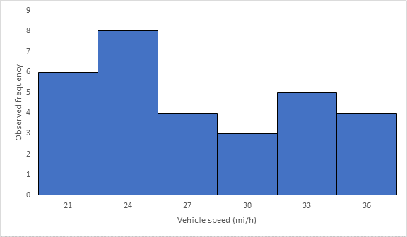
Below Figure shows the frequency histogram for the data shown in above Table. The values in columns 2 and 3 of Table are used to draw the frequency histogram, where the abscissa represents the speeds and the ordinate the observed frequency in each class.

Below Figure shows the cumulative frequency distribution curve for the data given. In this case, the cumulative percentages in column 6 of above Table are plotted against the upper limit of each corresponding speed class. This curve gives the percentage of vehicles that are traveling at or below a given speed.

Determine the arithmetic mean speed:
Conclusion:
The average speeds of each set of data are 34.9 and 27.5 mi/h respectively.
(b)
The histogram frequency distribution, cumulative percentage distribution for each set of data and 85th percentile speed.
Answer to Problem 10P
Explanation of Solution
Given:
Significance level of

Calculation:
Before an increase in speed enforcement activities:
The speed ranges from 28 to 40 mi/h giving a speed range of 12. For five classes, the range per class is 2.4 mi/h. A frequency distribution table can then be prepared, as shown below in which the speed classes are listed in column 1 and the mid-values are in column 2. The number of observations for each class is listed in column 3 and the cumulative percentages of all observations are listed in column 6.
| 1 | 2 | 3 | 4 | 5 | 6 | 7 |
| Speed class (mi/h) | Class mid-value | Class frequency, | Percentage of class frequency | Cumulative percentage of class frequency | ||
| 28-30 | 29 | 4 | 116 | 13 | 13 | 139.24 |
| 31-33 | 32 | 5 | 160 | 17 | 30 | 42.05 |
| 34-36 | 35 | 12 | 420 | 40 | 70 | 0.12 |
| 37-39 | 38 | 6 | 228 | 20 | 90 | 57.66 |
| 40-42 | 41 | 3 | 123 | 10 | 100 | 111.63 |
| Total | 30 | 1047 | 350.7 |
Below Figure shows the frequency histogram for the data shown in above Table. The values in columns 2 and 3 of Table are used to draw the frequency histogram, where the abscissa represents the speeds and the ordinate the observed frequency in each class.

Below Figure shows the cumulative frequency distribution curve for the data given. In this case, the cumulative percentages in column 6 of above Table are plotted against the upper limit of each corresponding speed class. This curve gives the percentage of vehicles that are traveling at or below a given speed.

The 85th-percentile speed is obtained from the cumulative frequency distribution curve as 36 mi/h.
After an increase in speed enforcement activities:
The speed ranges from 20 to 37 mi/h giving a speed range of 17. For six classes, the range per class is 2.83 mi/h. A frequency distribution table can then be prepared, as shown below in which the speed classes are listed in column 1 and the mid-values are in column 2. The number of observations for each class is listed in column 3 and the cumulative percentages of all observations are listed in column 6.
| 1 | 2 | 3 | 4 | 5 | 6 | 7 |
| Speed class (mi/h) | Class mid-value | Class frequency, | Percentage of class frequency | Cumulative percentage of class frequency | ||
| 20-22 | 21 | 6 | 126 | 20 | 20 | 253.5 |
| 23-25 | 24 | 8 | 192 | 27 | 47 | 98 |
| 26-28 | 27 | 4 | 108 | 13 | 60 | 1 |
| 29-31 | 30 | 3 | 90 | 10 | 70 | 18.75 |
| 32-34 | 33 | 5 | 165 | 17 | 87 | 151.25 |
| 35-37 | 36 | 4 | 144 | 13 | 100 | 289 |
| Total | 30 | 825 | 811.5 |
Below Figure shows the frequency histogram for the data shown in above Table. The values in columns 2 and 3 of Table are used to draw the frequency histogram, where the abscissa represents the speeds and the ordinate the observed frequency in each class.

Below Figure shows the cumulative frequency distribution curve for the data given. In this case, the cumulative percentages in column 6 of above Table are plotted against the upper limit of each corresponding speed class. This curve gives the percentage of vehicles that are traveling at or below a given speed.

The 85th-percentile speed is obtained from the cumulative frequency distribution curve as 31.5 mi/h.
Conclusion:
The 85th-percentile speed for each set of data are 36 and 31.5 mi/h respectively.
(c)
The histogram frequency distribution, cumulative percentage distribution for each set of data and 15th percentile speed.
Answer to Problem 10P
Explanation of Solution
Given:
Significance level of


Calculation:
Before an increase in speed enforcement activities:
The speed ranges from 28 to 40 mi/h giving a speed range of 12. For five classes, the range per class is 2.4 mi/h. A frequency distribution table can then be prepared, as shown below in which the speed classes are listed in column 1 and the mid-values are in column 2. The number of observations for each class is listed in column 3 and the cumulative percentages of all observations are listed in column 6.
| 1 | 2 | 3 | 4 | 5 | 6 | 7 |
| Speed class (mi/h) | Class mid-value | Class frequency, | Percentage of class frequency | Cumulative percentage of class frequency | ||
| 28-30 | 29 | 4 | 116 | 13 | 13 | 139.24 |
| 31-33 | 32 | 5 | 160 | 17 | 30 | 42.05 |
| 34-36 | 35 | 12 | 420 | 40 | 70 | 0.12 |
| 37-39 | 38 | 6 | 228 | 20 | 90 | 57.66 |
| 40-42 | 41 | 3 | 123 | 10 | 100 | 111.63 |
| Total | 30 | 1047 | 350.7 |
Below Figure shows the frequency histogram for the data shown in above Table. The values in columns 2 and 3 of Table are used to draw the frequency histogram, where the abscissa represents the speeds and the ordinate the observed frequency in each class.
Below Figure shows the cumulative frequency distribution curve for the data given. In this case, the cumulative percentages in column 6 of above Table are plotted against the upper limit of each corresponding speed class. This curve gives the percentage of vehicles that are traveling at or below a given speed.

The 15th-percentile speed is obtained from the cumulative frequency distribution curve as 28.5 mi/h.
After an increase in speed enforcement activities:
The speed ranges from 20 to 37 mi/h giving a speed range of 17. For six classes, the range per class is 2.83 mi/h. A frequency distribution table can then be prepared, as shown below in which the speed classes are listed in column 1 and the mid-values are in column 2. The number of observations for each class is listed in column 3 and the cumulative percentages of all observations are listed in column 6.
| 1 | 2 | 3 | 4 | 5 | 6 | 7 |
| Speed class (mi/h) | Class mid-value | Class frequency, | Percentage of class frequency | Cumulative percentage of class frequency | ||
| 20-22 | 21 | 6 | 126 | 20 | 20 | 253.5 |
| 23-25 | 24 | 8 | 192 | 27 | 47 | 98 |
| 26-28 | 27 | 4 | 108 | 13 | 60 | 1 |
| 29-31 | 30 | 3 | 90 | 10 | 70 | 18.75 |
| 32-34 | 33 | 5 | 165 | 17 | 87 | 151.25 |
| 35-37 | 36 | 4 | 144 | 13 | 100 | 289 |
| Total | 30 | 825 | 811.5 |
Below Figure shows the frequency histogram for the data shown in above Table. The values in columns 2 and 3 of Table are used to draw the frequency histogram, where the abscissa represents the speeds and the ordinate the observed frequency in each class.
Below Figure shows the cumulative frequency distribution curve for the data given. In this case, the cumulative percentages in column 6 of above Table are plotted against the upper limit of each corresponding speed class. This curve gives the percentage of vehicles that are traveling at or below a given speed.
The 15th-percentile speed is obtained from the cumulative frequency distribution curve as 0 mi/h.
Conclusion:
The 15th-percentile speed for each set of data are 28.5 and 0 mi/h respectively.
(d)
The histogram frequency distribution, cumulative percentage distribution for each set of data and mode.
Answer to Problem 10P
35 mi/h and 24 mi/h
Explanation of Solution
Given:
Significance level of


Calculation:
Before an increase in speed enforcement activities:
The speed ranges from 28 to 40 mi/h giving a speed range of 12. For five classes, the range per class is 2.4 mi/h. A frequency distribution table can then be prepared, as shown below in which the speed classes are listed in column 1 and the mid-values are in column 2. The number of observations for each class is listed in column 3 and the cumulative percentages of all observations are listed in column 6.
| 1 | 2 | 3 | 4 | 5 | 6 | 7 |
| Speed class (mi/h) | Class mid-value | Class frequency, | Percentage of class frequency | Cumulative percentage of class frequency | ||
| 28-30 | 29 | 4 | 116 | 13 | 13 | 139.24 |
| 31-33 | 32 | 5 | 160 | 17 | 30 | 42.05 |
| 34-36 | 35 | 12 | 420 | 40 | 70 | 0.12 |
| 37-39 | 38 | 6 | 228 | 20 | 90 | 57.66 |
| 40-42 | 41 | 3 | 123 | 10 | 100 | 111.63 |
| Total | 30 | 1047 | 350.7 |
Below Figure shows the frequency histogram for the data shown in above Table. The values in columns 2 and 3 of Table are used to draw the frequency histogram, where the abscissa represents the speeds and the ordinate the observed frequency in each class.

Below Figure shows the cumulative frequency distribution curve for the data given. In this case, the cumulative percentages in column 6 of above Table are plotted against the upper limit of each corresponding speed class. This curve gives the percentage of vehicles that are traveling at or below a given speed.

The mode or modal speed is obtained from the frequency histogram as 35 mi/h
After an increase in speed enforcement activities:
The speed ranges from 20 to 37 mi/h giving a speed range of 17. For six classes, the range per class is 2.83 mi/h. A frequency distribution table can then be prepared, as shown below in which the speed classes are listed in column 1 and the mid-values are in column 2. The number of observations for each class is listed in column 3 and the cumulative percentages of all observations are listed in column 6.
| 1 | 2 | 3 | 4 | 5 | 6 | 7 |
| Speed class (mi/h) | Class mid-value | Class frequency, | Percentage of class frequency | Cumulative percentage of class frequency | ||
| 20-22 | 21 | 6 | 126 | 20 | 20 | 253.5 |
| 23-25 | 24 | 8 | 192 | 27 | 47 | 98 |
| 26-28 | 27 | 4 | 108 | 13 | 60 | 1 |
| 29-31 | 30 | 3 | 90 | 10 | 70 | 18.75 |
| 32-34 | 33 | 5 | 165 | 17 | 87 | 151.25 |
| 35-37 | 36 | 4 | 144 | 13 | 100 | 289 |
| Total | 30 | 825 | 811.5 |
Below Figure shows the frequency histogram for the data shown in above Table. The values in columns 2 and 3 of Table are used to draw the frequency histogram, where the abscissa represents the speeds and the ordinate the observed frequency in each class.

Below Figure shows the cumulative frequency distribution curve for the data given. In this case, the cumulative percentages in column 6 of above Table are plotted against the upper limit of each corresponding speed class. This curve gives the percentage of vehicles that are traveling at or below a given speed.

The mode or modal speed is obtained from the frequency histogram as 24 mi/h.
Conclusion:
The mode for each set of data are 35 and 24 mi/h respectively.
(e)
The histogram frequency distribution, cumulative percentage distribution for each set of data and median.
Answer to Problem 10P
32.5 and 23.5 mi/h
Explanation of Solution
Given:
Significance level of


Calculation:
Before an increase in speed enforcement activities:
The speed ranges from 28 to 40 mi/h giving a speed range of 12. For five classes, the range per class is 2.4 mi/h. A frequency distribution table can then be prepared, as shown below in which the speed classes are listed in column 1 and the mid-values are in column 2. The number of observations for each class is listed in column 3 and the cumulative percentages of all observations are listed in column 6.
| 1 | 2 | 3 | 4 | 5 | 6 | 7 |
| Speed class (mi/h) | Class mid-value | Class frequency, | Percentage of class frequency | Cumulative percentage of class frequency | ||
| 28-30 | 29 | 4 | 116 | 13 | 13 | 139.24 |
| 31-33 | 32 | 5 | 160 | 17 | 30 | 42.05 |
| 34-36 | 35 | 12 | 420 | 40 | 70 | 0.12 |
| 37-39 | 38 | 6 | 228 | 20 | 90 | 57.66 |
| 40-42 | 41 | 3 | 123 | 10 | 100 | 111.63 |
| Total | 30 | 1047 | 350.7 |
Below Figure shows the frequency histogram for the data shown in above Table. The values in columns 2 and 3 of Table are used to draw the frequency histogram, where the abscissa represents the speeds and the ordinate the observed frequency in each class.

Below Figure shows the cumulative frequency distribution curve for the data given. In this case, the cumulative percentages in column 6 of above Table are plotted against the upper limit of each corresponding speed class. This curve gives the percentage of vehicles that are traveling at or below a given speed.

The median speed is obtained from the cumulative frequency distribution curve as 32.5 mi/h which is the 50th percentile speed.
After an increase in speed enforcement activities:
The speed ranges from 20 to 37 mi/h giving a speed range of 17. For six classes, the range per class is 2.83 mi/h. A frequency distribution table can then be prepared, as shown below in which the speed classes are listed in column 1 and the mid-values are in column 2. The number of observations for each class is listed in column 3 and the cumulative percentages of all observations are listed in column 6.
| 1 | 2 | 3 | 4 | 5 | 6 | 7 |
| Speed class (mi/h) | Class mid-value | Class frequency, | Percentage of class frequency | Cumulative percentage of class frequency | ||
| 20-22 | 21 | 6 | 126 | 20 | 20 | 253.5 |
| 23-25 | 24 | 8 | 192 | 27 | 47 | 98 |
| 26-28 | 27 | 4 | 108 | 13 | 60 | 1 |
| 29-31 | 30 | 3 | 90 | 10 | 70 | 18.75 |
| 32-34 | 33 | 5 | 165 | 17 | 87 | 151.25 |
| 35-37 | 36 | 4 | 144 | 13 | 100 | 289 |
| Total | 30 | 825 | 811.5 |
Below Figure shows the frequency histogram for the data shown in above Table. The values in columns 2 and 3 of Table are used to draw the frequency histogram, where the abscissa represents the speeds and the ordinate the observed frequency in each class.

Below Figure shows the cumulative frequency distribution curve for the data given. In this case, the cumulative percentages in column 6 of above Table are plotted against the upper limit of each corresponding speed class. This curve gives the percentage of vehicles that are traveling at or below a given speed.

The median speed is obtained from the cumulative frequency distribution curve as 23.5 mi/h which is the 50th percentile speed.
Conclusion:
The median speed for each set of data are 32.5 and 23.5 mi/h respectively.
(f)
The histogram frequency distribution, cumulative percentage distribution for each set of data and pace.
Answer to Problem 10P
32 to 39 mi/h and 27 to 36 mi/h
Explanation of Solution
Given:
Significance level of


Calculation:
Before an increase in speed enforcement activities:
The speed ranges from 28 to 40 mi/h giving a speed range of 12. For five classes, the range per class is 2.4 mi/h. A frequency distribution table can then be prepared, as shown below in which the speed classes are listed in column 1 and the mid-values are in column 2. The number of observations for each class is listed in column 3 and the cumulative percentages of all observations are listed in column 6.
| 1 | 2 | 3 | 4 | 5 | 6 | 7 |
| Speed class (mi/h) | Class mid-value | Class frequency, | Percentage of class frequency | Cumulative percentage of class frequency | ||
| 28-30 | 29 | 4 | 116 | 13 | 13 | 139.24 |
| 31-33 | 32 | 5 | 160 | 17 | 30 | 42.05 |
| 34-36 | 35 | 12 | 420 | 40 | 70 | 0.12 |
| 37-39 | 38 | 6 | 228 | 20 | 90 | 57.66 |
| 40-42 | 41 | 3 | 123 | 10 | 100 | 111.63 |
| Total | 30 | 1047 | 350.7 |
Below Figure shows the frequency histogram for the data shown in above Table. The values in columns 2 and 3 of Table are used to draw the frequency histogram, where the abscissa represents the speeds and the ordinate the observed frequency in each class.

Below Figure shows the cumulative frequency distribution curve for the data given. In this case, the cumulative percentages in column 6 of above Table are plotted against the upper limit of each corresponding speed class. This curve gives the percentage of vehicles that are traveling at or below a given speed.
Below figure shows the frequency distribution curve for the data given. In this case, a curve showing percentage of observations against speed is drawn by plotting values from column 5 of above Table against the corresponding values in column 2. The total area under this curve is one or 100 percent.
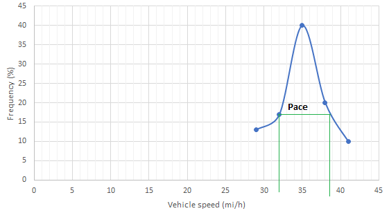
The pace is obtained from the frequency distribution curve above as 32 to 39 mi/h.
After an increase in speed enforcement activities:
The speed ranges from 20 to 37 mi/h giving a speed range of 17. For six classes, the range per class is 2.83 mi/h. A frequency distribution table can then be prepared, as shown below in which the speed classes are listed in column 1 and the mid-values are in column 2. The number of observations for each class is listed in column 3 and the cumulative percentages of all observations are listed in column 6.
| 1 | 2 | 3 | 4 | 5 | 6 | 7 |
| Speed class (mi/h) | Class mid-value | Class frequency, | Percentage of class frequency | Cumulative percentage of class frequency | ||
| 20-22 | 21 | 6 | 126 | 20 | 20 | 253.5 |
| 23-25 | 24 | 8 | 192 | 27 | 47 | 98 |
| 26-28 | 27 | 4 | 108 | 13 | 60 | 1 |
| 29-31 | 30 | 3 | 90 | 10 | 70 | 18.75 |
| 32-34 | 33 | 5 | 165 | 17 | 87 | 151.25 |
| 35-37 | 36 | 4 | 144 | 13 | 100 | 289 |
| Total | 30 | 825 | 811.5 |
Below Figure shows the frequency histogram for the data shown in above Table. The values in columns 2 and 3 of Table are used to draw the frequency histogram, where the abscissa represents the speeds and the ordinate the observed frequency in each class.

Below Figure shows the cumulative frequency distribution curve for the data given. In this case, the cumulative percentages in column 6 of above Table are plotted against the upper limit of each corresponding speed class. This curve gives the percentage of vehicles that are traveling at or below a given speed.

Below figure shows the frequency distribution curve for the data given. In this case, a curve showing percentage of observations against speed is drawn by plotting values from column 5 of above Table against the corresponding values in column 2. The total area under this curve is one or 100 percent.
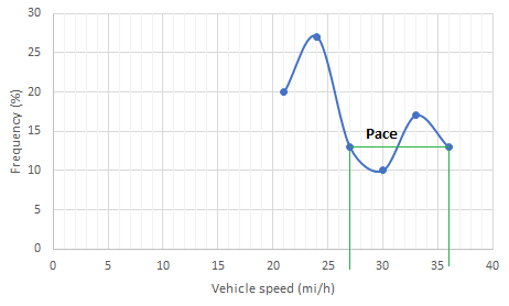
The pace is obtained from the frequency distribution curve drawn above as 27 to 36 mi/h.
Conclusion:
The pace for each set of data are 32 to 39 mi/h and 27 to 36 mi/h respectively.
Want to see more full solutions like this?
Chapter 4 Solutions
EBK TRAFFIC AND HIGHWAY ENGINEERING


- Traffic data are collected in 60-second intervals at a specific highway location as shown in the Table. Assuming the traffic arrivals are Poisson distributed and continue at the same rate as that observed in the 15 time periods shown, what is the probability that six or more vehicles will arrive in each of the next three 60-second time intervals (12:15 P.M. to 12:16 P.M., 12:16 P.M. to 12:17 P.M., and 12:17 P.M. to 12:18 P.M.)?arrow_forwardGiven that the value of a segment of a roadway is 720 veh/hr where arrival of vehicles is a poisson distribution. Calculate the following: a. No. of headways if it is less than 5 seconds b. No. of headways if it is more than 5 seconds c. Plot the probability curves of the 2 conditions stated above.arrow_forwardThis is a three-part question. Data obtained from aerial photography showed eight vehicles on an 800 ft-long section of road. Traffic data collected at the same time indicated an average time headway of 3.7 sec. Part A. Determine the density on the highway in vehicles per mile. Part B. Determine the flow on the road in vehicles per hour. Part C. Determine the space mean speed in mph.arrow_forward
- What is the probability that time headway is greater than or equal to 2 sec? Assume arrival rate of vehicle follows Poisson's distribution curve.arrow_forwardIn The entrance of car parking, The vehicle arrival in each counting period of 100 sec. is shown in Table below, check whether The arrival distribution of vehicle can be assumed random or not vehicle per 100 sec 0 1 2 3 >= 4 frequency 60 28 16 8 0arrow_forwardVehicles arrive at an entrance to a recreational park. There is a single gate (at which all vehicles must stop), where a park attendant distributes a free brochure. The park opens at 8:00 A.M., the average arrival rate be 240 veh/h and Poisson distributed (exponential times between arrivals) over the entire period from park opening time (8:00 A.M.) until closing at dusk. If the time required to distribute the brochure is 10 seconds, the distribution time varies depending on whether park patrons have questions relating to park operating policies, assuming M/M/1 queuing. a.) Compute the average length of queue (express in veh), b.) Average waiting time in the queue (express in min/veh), c.) and average time spent in the system(express in min/veh)arrow_forward
- Consider the following spot speed data, which were collected from the location of expressways operating under free flow conditions: a. Draw the frequency curve and cumulative frequency for this data. b. Find and identify on the curve: average speed, modud speed, pace, percent of vehicles in pace. c. Calculate the mean and standard deviation of the velocity distribution. d. What are the confidence bounds in the true mean velocity estimate of the underlying distribution with a 95% confidence level? With a 99.7% confidence level? e. Based on the results of this study, a second study should be conducted to achieve a tolerance of ±1.5 mi/hour with a 95% confidence level. What is the required sample size? f. Can this data deserve to be declared as normal?arrow_forward. A traffic enforcer counts the number of vehicles at a specific location in the highway. In hiscounting, there are 420 vehicles arrived in span of 1 hour. Assuming that the arrival of vehicles isPoisson distributed, estimate the probabilities of having 7 or more vehicles arriving over a 30-secondtime intervalarrow_forwardAt a specified point on a highway, vehicles are known to arrive according to a Poisson process. Vehicles are counted in 20-second intervals, and vehicle counts are taken in 120 of these time intervals. It is noted that no cars arrive in 18 of these 120 intervals. Approximate the number of these 120 intervals in which exactly three cars arrive. Wrong answers will be downvoted read question carefullyarrow_forward
- The time between arrivals of vehicles at a particular intersection follows an exponential probability distribution with a mean of 14 seconds. A. What is the probability that the arrival time between vehicles is 12 seconds or less (to 4 decimals)? B. What is the probability that the arrival time between vehicles is 6 seconds or less (to 4 decimals)? C. What is the probability of 30 or more seconds between vehicle arrivals (to 4 decimals)?arrow_forwardIn the plot of cumulative vehicle arrivals and cumulative vehicle departure curves (y-axis) vs. time (x-axis), the queue disappears when: Group of answer choices The cumulative arrival = cumulative departure The cumulative departure = 0 The cumulative arrival = 0 The departure rate (or service rate) > arrival ratearrow_forwardA) A traffic engineer records the travel times of vehicles as they traveled a 1.0-mile segment of highway during (1.2, 1.25, 1.6, 1.5, 1.8, and 1.5 minutes). Find space mean speed (SMS) and time mean speed (TMS).arrow_forward
 Traffic and Highway EngineeringCivil EngineeringISBN:9781305156241Author:Garber, Nicholas J.Publisher:Cengage Learning