
Videos
For its first 2 decades of existence, the NBA’s Orlando Magic basketball team set seat prices for its 41-game home
But when Anthony Perez, director of business strategy, finished his MBA at the University of Florida, he developed a valuable database of ticket sales. Analysis of the data led him to build a
Studying individual sales of Magic tickets on the open Stub Hub marketplace during the prior season, Perez determined the additional potential sales revenue the Magic could have made had they charged prices the fans had proven they were willing to pay on Stub Hub. This became his dependent variable, y, in a multiple-regression model.
He also found that three variables would help him build the “true market” seat price for every game. With his model, it was possible that the same seat in the arena would have as many as seven different prices created at season onset—sometimes higher than expected on average and sometimes lower.
The major factors he found to be statistically significant in determining how high the demand for a game ticket, and hence, its price, would be were:
► The day of the week (x1)
► A rating of how popular the opponent was (x2)
► The time of the year (x3)
For the day of the week, Perez found that Mondays were the least-favored game days (and he assigned them a value of 1). The rest of the weekdays increased in popularity, up to a Saturday game, which he rated a 6. Sundays and Fridays received 5 ratings, and holidays a 3 (refer to the footnote in Table 4.2).

Fernado Medina
TABLE 4.2 Data for Last Year’s Magic Ticket Sales Pricing Model
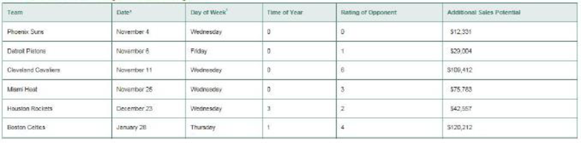
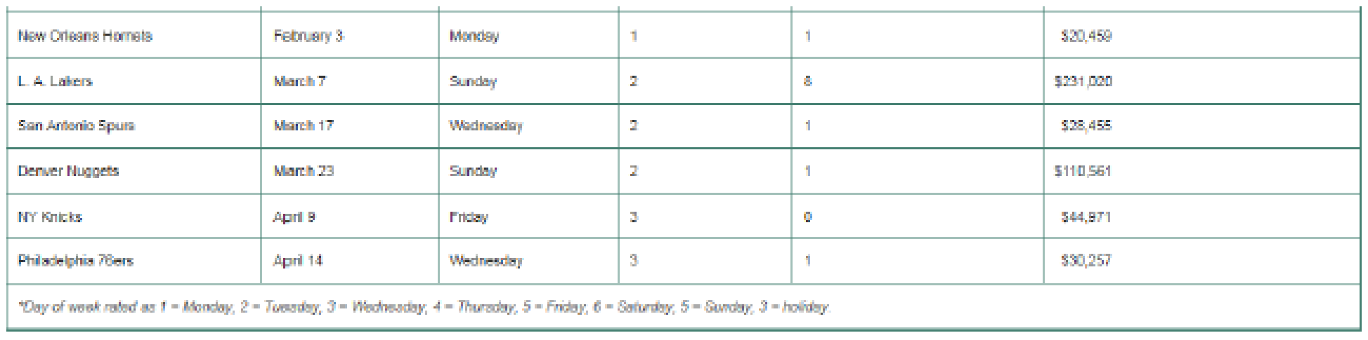
His ratings of opponents, done just before the start of the season, were subjective and range from a low of 0 to a high of 8. A very high-rated team in that particular season may have had one or more superstars on its roster, or have won the NBA finals the prior season, making it a popular fan draw.
Finally, Perez believed that the NBA season could be divided into four periods in popularity:
► Early games (which he assigned 0 scores)
► Games during the Christmas season (assigned a 3)
► Games until the All-Star break (given a 2)
► Games leading into the play-offs (scored with a 3)
The first year Perez built his multiple-regression model, the dependent variable y, which was a “potential premium revenue score,” yielded an R2 =.86 with this equation:
Table 4.2 illustrates, for brevity in this case study, a sample of 12 games that year (out of the total 41 home game regular season), including the potential extra revenue per game (y) to be expected using the variable pricing model.
A leader in NBA variable pricing, the Orlando Magic have learned that regression analysis is indeed a profitable forecasting tool.
1. Use the data in Table 4.2 to build a regression model with day of the week as the only independent variable.
4. What additional independent variables might you suggest to include in Perez’s model?
Want to see the full answer?
Check out a sample textbook solution
Chapter 4 Solutions
OPERATIONS MGMT(LOOSELEAF)W/MYOMLAB>IC


- At the beginning of each week, a machine is in one of four conditions: 1 = excellent; 2 = good; 3 = average; 4 = bad. The weekly revenue earned by a machine in state 1, 2, 3, or 4 is 100, 90, 50, or 10, respectively. After observing the condition of the machine at the beginning of the week, the company has the option, for a cost of 200, of instantaneously replacing the machine with an excellent machine. The quality of the machine deteriorates over time, as shown in the file P10 41.xlsx. Four maintenance policies are under consideration: Policy 1: Never replace a machine. Policy 2: Immediately replace a bad machine. Policy 3: Immediately replace a bad or average machine. Policy 4: Immediately replace a bad, average, or good machine. Simulate each of these policies for 50 weeks (using at least 250 iterations each) to determine the policy that maximizes expected weekly profit. Assume that the machine at the beginning of week 1 is excellent.arrow_forwardThe Tinkan Company produces one-pound cans for the Canadian salmon industry. Each year the salmon spawn during a 24-hour period and must be canned immediately. Tinkan has the following agreement with the salmon industry. The company can deliver as many cans as it chooses. Then the salmon are caught. For each can by which Tinkan falls short of the salmon industrys needs, the company pays the industry a 2 penalty. Cans cost Tinkan 1 to produce and are sold by Tinkan for 2 per can. If any cans are left over, they are returned to Tinkan and the company reimburses the industry 2 for each extra can. These extra cans are put in storage for next year. Each year a can is held in storage, a carrying cost equal to 20% of the cans production cost is incurred. It is well known that the number of salmon harvested during a year is strongly related to the number of salmon harvested the previous year. In fact, using past data, Tinkan estimates that the harvest size in year t, Ht (measured in the number of cans required), is related to the harvest size in the previous year, Ht1, by the equation Ht = Ht1et where et is normally distributed with mean 1.02 and standard deviation 0.10. Tinkan plans to use the following production strategy. For some value of x, it produces enough cans at the beginning of year t to bring its inventory up to x+Ht, where Ht is the predicted harvest size in year t. Then it delivers these cans to the salmon industry. For example, if it uses x = 100,000, the predicted harvest size is 500,000 cans, and 80,000 cans are already in inventory, then Tinkan produces and delivers 520,000 cans. Given that the harvest size for the previous year was 550,000 cans, use simulation to help Tinkan develop a production strategy that maximizes its expected profit over the next 20 years. Assume that the company begins year 1 with an initial inventory of 300,000 cans.arrow_forward
 Practical Management ScienceOperations ManagementISBN:9781337406659Author:WINSTON, Wayne L.Publisher:Cengage,