
(a)
Estimated regression line.
(a)
Explanation of Solution
The formula for the regression equation is:
Run the ordinary least squares method for the given data in excel. The results drawn are as follows:
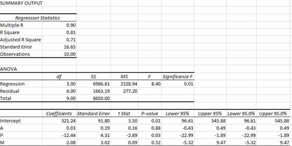
Use the summary output to find the estimated regression equation as follows:
(b)
The economic interpretation of the estimated intercept (a) and slope (b) coefficients.
(b)
Explanation of Solution
Interpretation of estimated intercept (a) coefficient:
When the selling price, promotional expenditure and disposable income are zero, on average the quantity sold of pens is equal to 321.24× $1000 = $321,240.
Interpretation of estimated slope (b) coefficient:
For a given level of selling price and disposable income, an additional $1,000 promotional expenditures lead to a rise in sales by 0.03×1000 = 30 gallons on average.
For a given level of promotional expenditure and selling price, an additional $1,000 disposable income leads to a rise in sales by 2.08×1000 = 2,080 gallons on an average.
For a given level of promotional expenditure and disposable income, an additional $1/gallon lead to falling in sales by 12.44×1000 = 12,440 gallons on an average.
(c)
The hypothesis that there is no relationship between the variables at 0.05 significance level.
(c)
Explanation of Solution
Conduct the t-test to know the statistical significance of the independent variables A, Pand M. The test statistic can be calculated using the following formula:
The t-statistic follows t-distribution with n-1 degrees of freedom.
For variable A, t-test is conducted as follows:
According to the summary output, the t-statistic for A variable is equal to 0.16.
At 5% significance level and 10-1=9 degrees of freedom, the critical value is equal to 2.262.
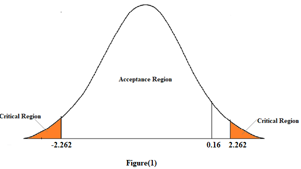
In figure (1), since the calculated t-statistic lies in the acceptance region. Therefore, we accept the null hypothesis. This means that the variable A is not statistically significant.
For variable P, t-test is conducted as follows:
According to the summary output, the t-statistic for P variable is equal to -2.89. At 5% significance level and 10-1=9 degrees of freedom, the critical value is equal to 2.262.
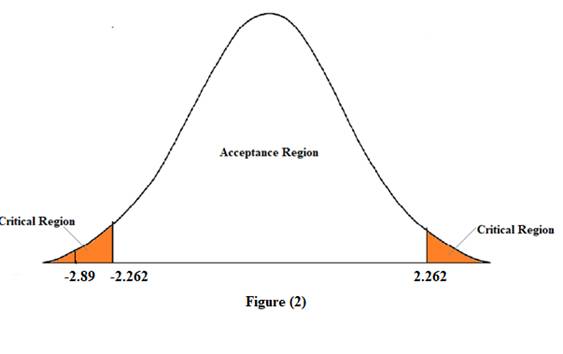
In figure (2), since the calculated t-statistic lies in the critical region. Therefore, we reject the null hypothesis. This means that the variable Pis statistically significant.
For variable M, t-test is conducted as follows:
According to the summary output, the t-statistic for M variable is equal to 0.69.
At 5% significance level and 10-1=9 degrees of freedom, the critical value is equal to 2.262.
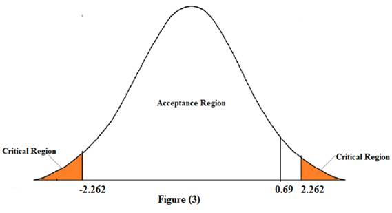
In figure (3), since the calculated t-statistic lies in the acceptance region. Therefore, we accept the null hypothesis. This means that the M variable is not statistically significant.
(d)
Coefficient of determination.
(d)
Explanation of Solution
The coefficient of determination measures the proportion of variance predicted by the independent variable in the dependent variable. It is denoted as R2.
According to the summary output, the value of R2 is equal to 0.81. This means that the regression equation predicts 81% of the variance in sales.
(e)
Analysis of variance on the regression including F-test of the overall significance of the results.
(e)
Explanation of Solution
The value of F-statistic is given as 8.40. And the critical value at 0.05 significance level is equal to 0.01.
Since F-statistic is greater than the critical value, thus, the overall model is statistically significant.
(f)
Best estimate of the product sales when the selling price is $14.50. And an approximate 95 percent prediction interval.
(f)
Explanation of Solution
According to the regression statistics of the summary output, for a given level of promotional expenditure and disposable income, $14.50/gallon lead to fall in sales by 12.44×14.50×1000 = 180,380 gallons on an average.
According to the regression statistics in the summary output, a 95% confidence interval for the P variable ranges from -22.99 to -1.89.
(g)
Price elasticity of demand at a selling price of $14.50.
(g)
Explanation of Solution
Formula to calculate elasticity in linear regression model is as follows:
At given value of P variable equal to 14.50, the estimated value of Y variable is equal to 180,380.
Thus, price elasticity of demand is calculated as follows:
Thus, the price elasticity of demand at a selling price of $14.50 is equal to -0.001.
Want to see more full solutions like this?
Chapter 4 Solutions
Managerial Economics: Applications, Strategies and Tactics (MindTap Course List)

- Suppose the Sherwin-Williams Company has developed the following multiple regression model, with paint sales Y (x 1,000 gallons) as the dependent variable and promotional expenditures A (x $1,000) and selling price P (dollars per gallon) as the independent variables. Y=α+βaA+βpP+εY=α+βaA+βpP+ε Now suppose that the estimate of the model produces following results: α=344.585α=344.585, ba=0.102ba=0.102, bp=−11.192bp=−11.192, sba=0.173sba=0.173, sbp=4.487sbp=4.487, R2=0.813R2=0.813, and F-statistic=11.361F-statistic=11.361. Note that the sample consists of 10 observations. 1.) According to the estimated model, holding all else constant, a $1,000 increase in promotional expenditures decrease or increase sales by approximately 102,813 or 11,192 gallons. Similarly, a $1 increase in the selling price decrease or increase sales by approximately 813,11,192 or 102 gallons. 2.)Which of the independent variables (if any) appears to be statistically significant (at the 0.05…arrow_forwardXYZ company is interested in quantifying the impact of consumer promotions on the sales of its packaged food product. XYZ has historical data on the following variables for 38 weeks: • Sales: Weekly sales volume in thousands of units.• Prom: Weekly spending on consumer promotions in thousands of Dollars" "A regression analysis was applied to XYZ historical dataset. The dependent variable is weekly Sales and the independent variables are weekly Prom and weekly Lagged Prom (i.e., last week Prom). This is a summary of the regression output:Sales = 0.80 + 1.20*Prom - 0.40*Lag(Prom) • R-squared=0.85• F-Statistic=23.83• p-value=0.001 (for the overall regression)•All regression coefficients are statistically significant at the 5% level." A. What will be the predicted sales volume ? B. What is the gross margin of this net volume impact due to $1000 spending per week on consumer promotions, if brand makes $2.20 gross margin per unit . C. What is the ROI of this promotion? D. What is predicted…arrow_forwardWhich of the following is a consequence of severe multicollinearity in a regression model? A. High standard errors for the estimated coefficientsB. Lower standard errors for the estimated coefficientsC. The OLS estimator becomes biasedD. The dependent variable becomes constantarrow_forward
- General Cereals is using a regression model to estimate the demand for Tweetie Sweeties, a whistle-shaped, sugar-coated breakfast cereal for children. The following (multiplicative exponential) demand function is being used: QD=6,280 P(−1.85)A2.05N2.70QD=6,280 P−1.85A2.05N2.70 where QDQD = quantity demanded, in 10-oz boxes PP = price per box, in dollars AA = advertising expenditures on daytime television, in dollars NN = proportion of the population under 12 years old, in percent What is the point price elasticity of demand for Tweetie Sweeties? 2.05 2.70 -0.90 -1.85 What is the advertising elasticity of demand? 0.76 -1.85 2.70 2.05arrow_forwardIn a regression problem with 1 output variable and with a total number of 100 possible input variables, what is the number of all possible models with three input variables?arrow_forwardIn a regression problem with one output variable and one input variable, we set up two cutpoints z1 and z2 for the input variable and we fit a step function regression model based on these two cutpoints of the input variable. If you write the regression problem in matrix form y = X%*%β + ε, how many rows would the vector β have?arrow_forward
- Q. Wilpen Company, a price-setting firm, produces nearly 80 percent of all tennis balls purchased in the United States. Wilpen estimates the U.S. demand for its tennis balls by using the following linear specification: Q = a + bP + cM + dPR. Where Q is the number of cans of tennis balls sold quarterly, P is the wholesale price Wilpen charges for a can of tennis balls, M is the consumers’ average household income, and PR is the average price of tennis rackets. The regression results are as follows: a- Discuss the statistical significance of the parameter estimates a^, b^, c^, and d^ using the p-values. Are the signs of b^, c^, and d^ consistent with the theory of demand? Wilpen plans to charge a wholesale price of $1.65 per can. The average price of a tennis racket is $110, and consumers’ average household income is $24,600. b. What is the estimated number of cans of tennis balls demanded? c) At the values of P, M, and Pr given, what are the estimated values of the price (E^), income…arrow_forwardQ. Wilpen Company, a price-setting firm, produces nearly 80 percent of all tennis balls purchased in the United States. Wilpen estimates the U.S. demand for its tennis balls by using the following linear specification: Q = a + bP + cM + dPR. Where Q is the number of cans of tennis balls sold quarterly, P is the wholesale price Wilpen charges for a can of tennis balls, M is the consumers’ average household income, and PR is the average price of tennis rackets. The regression results are as follows: a. Discuss the statistical significance of the parameter estimates a^, b^, c^, and d^ using the p-values. Are the signs of b^, c^, and d^ consistent with the theory of demand? Wilpen plans to charge a wholesale price of $1.65 per can. The average price of a tennis racket is $110, and consumers’ average household income is $24,600. b. What is the estimated number of cans of tennis balls demanded? c) At the values of P, M, and Pr given, what are the estimated values of the price (E^), income…arrow_forwardThe following data relate the sales figures of the bar in Mark Kaltenbach's small bed-and-breakfast inn in portland, to the number of guest registered that week: week guests bar sales 1 16 $330 2 12 $270 3 18 $380 4 14 $315 a) The simple linear regression equation that relates bar sales to number of guests(not to time) is (round your responses to one decimal place): Bar sales = [___]+[___]X guestsarrow_forward
- 1.1 Which of the following is NOT a good reason for including a disturbance term in a regression equation?/ A. To allow for random influences on the dependent variable/ B. To allow for errors in the measurement of the dependent variable/ C. It captures omitted determinants of the dependent variable D. To allow for the non-zero mean of the dependent variable/ 1.2 Consider the equation Y = B1 + B2X2 + u. A null hypothesis of H0: B2 = 0 means that/ A. X2 has no effect on the expected value of Y / B. B2 has no effect on the expected value of Y/ C. X2 has no effect on the expected value of B2 / D. Y has no effect on the expected value of X2/ 1.3 The OLS residuals in the multiple regression model/ A. can be calculated by subtracting the fitted values from the actual values / B. are zero because the predicted values are another name for forecasted values / C. are typically the same as the population regression function errors / D. cannot be calculated because there…arrow_forwardWhich of the following are plausible approaches to dealing with a model that exhibits heteroscredasticity? i) Take logarithms of each of the variables ii) Use suitably modified standart errors iii) Use generalised least squares procedure iv) Add lagged values of the variables to the regression equation Answers: a- (i), (ii), (iii) and (iv) b- (ii) and (iv) c- (i) and (iii) d- (i), (ii) and (iii) What is the answer?arrow_forwardA simple regression analysis to estimate the demand for Chick-fil-A’s new premium super-sized spicy chicken sandwich is Q= 48-2p. If Chick-fil-A sets the price at $12 and Q=20, calculate the regression’s error term? Also, list five assumptions of the classical linear regression model.arrow_forward
 Managerial Economics: Applications, Strategies an...EconomicsISBN:9781305506381Author:James R. McGuigan, R. Charles Moyer, Frederick H.deB. HarrisPublisher:Cengage Learning