
Videos
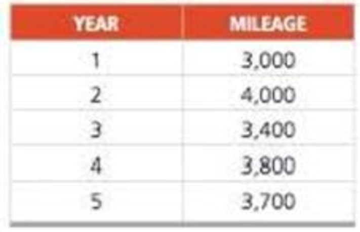
The Carbondale Hospital is considering the purchase of a new ambulance. The decision will rest partly on the anticipated mileage to be driven next year. The miles driven during the past 5 years are as follows:
a) Forecast the mileage for next year (6th year) using a 2-year moving average.
b) Find the MAD based on the 2-year moving average. (Hint: You will have only 3 years of matched data.)
c) Use a weighted 2-year moving average with weights of .4 and .6 to forecast next year’s mileage. (The weight of .6 is for the most recent year.) What MAD results from using this approach to
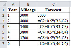
d) Compute the forecast for year 6 using exponential smoothing, an initial forecast for year 1 of 3,000 miles, and α = .5.
a)
To determine: Using 2-year moving average, forecast the mileage for the 6th year.
Introduction: Forecasting is used to predict future changes or demand patterns. It involves different approaches and varies with different time periods. A sequence of data points in successive order is known as a time series. Time series forecasting is the prediction based on past events which are at a uniform time interval.
Answer to Problem 5P
The forecasted mileage for the 6th year is 3,750.
Explanation of Solution
Given information:
| Year | Mileage |
| 1 | 3,000 |
| 2 | 4,000 |
| 3 | 3,400 |
| 4 | 3,800 |
| 5 | 3,700 |
Formula to forecast the mileage for the 6th year:
| Year | Mileage | Moving Average |
| 1 | 3,000 | |
| 2 | 4,000 | |
| 3 | 3,400 | 3,500 |
| 4 | 3,800 | 3,700 |
| 5 | 3,700 | 3,600 |
| 6 | 3,750 |
Excel worksheet:
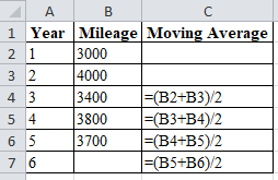
Calculation of the mileage forecast for the 6th year:
The mileage forecast for the 6th year is obtained by summing up the mileage for the 4th and 5thyears and dividing the sum by the
The forecast for the 6th year is 3,750.
Hence, using 2-year moving average, the mileage forecast for the 6th year is 3,750
b)
To determine: The computation of the Mean Average Deviation (MAD) using 2-year moving average.
Answer to Problem 5P
Mean Average Deviation (MAD) using 2-year moving average is 100
Explanation of Solution
Given information:
| Year | Mileage |
| 1 | 3,000 |
| 2 | 4,000 |
| 3 | 3,400 |
| 4 | 3,800 |
| 5 | 3,700 |
Formula to compute MAD:
| Year | Mileage | Moving Average | Error | Absolute Error |
| 1 | 3,000 | |||
| 2 | 4,000 | |||
| 3 | 3,400 | 3,500 | -100 | 100 |
| 4 | 3,800 | 3,700 | 100 | 100 |
| 5 | 3,700 | 3,600 | 100 | 100 |
| Total | 300 | |||
| MAD | 100 |
Excel worksheet:
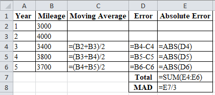
Calculation of the absolute error for year 3:
Moving average:
Error:
Absolute error:
To calculate the forecast for year 3, divide the summation of the values of year 1&2 by period n i.e. 2. The corresponding value is 3500 which is the forecast for the year 3.
Absolute Error for year 3 is the modulus of the difference between 3400 and 3500, which corresponds to 100. Therefore absolute error for year 3 is 100.
Calculation of the absolute error for year 4:
Moving average:
Error:
Absolute error:
To calculate the forecast for year 4, divide the summation of the values of year 2&3 by period n i.e. 2. The corresponding value is 3700 which is the forecast for the year 4.
Absolute Error for year 4 is the modulus of the difference between 3800 & 3700 which corresponds to 100. Therefore Absolute error for Year 4 is 100.
Calculation of the absolute error for year 5:
Moving average:
Error:
Absolute error:
To calculate the forecast for year 5, divide the summation of the values of year 3&4 by period n i.e. 2. The corresponding value is 3600 which is the forecast for the year 5.
Absolute Error for year 5 is the modulus of the difference between 3,700 & 3,600 which corresponds to 100. Therefore Absolute error for Year 5 is 100.
Calculation of the Mean Absolute Deviation:
Mean Absolute Deviation is obtained by dividing the summation of absolute values by the number of years. Absolute error is obtained by taking modulus for the difference between Actual and forecasted values.
Upon substitution of summation value of absolute error for 3 years i.e. 300 is divided by number of years i.e. 3 yields MAD of 100.
Hence, the computed Mean Average Deviation (MAD) using 2-year moving average is 100
c)
To determine: The mileage forecast for year 6 and also compute Mean Absolute Deviation (MAD) using weighted 2-year moving average with weights 0.4 and 0.6
Answer to Problem 5P
The forecast for year 6 and the Mean Absolute Deviation (MAD) using weighted moving averages are 3,741 & 139.67 respectively.
Explanation of Solution
Given information:
| Year | Mileage |
| 1 | 3,000 |
| 2 | 4,000 |
| 3 | 3,400 |
| 4 | 3,800 |
| 5 | 3,700 |
Formula to compute MAD:
| Year | Mileage | Weighted Moving Average | Error | Absolute Error |
| 1 | 3,000 | |||
| 2 | 4,000 | |||
| 3 | 3,400 | 3,601 | -201 | 201 |
| 4 | 3,800 | 3,641 | 159 | 159 |
| 5 | 3,700 | 3,641 | 59 | 59 |
| 6 | 3,741 | |||
| Total | 419 | |||
| MAD | 139.67 |
Excel worksheet:
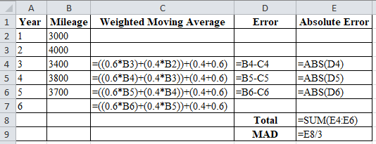
Calculation of the weighted moving average for year 3:
To calculate the forecast for year 3, multiply the weights with the mileage of recent year, i.e. multiply weight 0.6 with 4,000 and 0.4 with 3,000. Divide the summation of the multiplied values with the summation of the weights i.e. (0.6+0.4).
The corresponding result is 3,601 obtained is the forecasted value for year 3. Therefore, forecasted Weighted Moving Average for year 3 is 3,601.
Calculation of the weighted moving average for year 4:
To calculate the forecast for year 4, multiply the weights with the mileage of recent year, i.e. multiply weight 0.6 with 3,400 and 0.4 with 4,000. Divide the summation of the multiplied values with the summation of the weights i.e. (0.6+0.4).
The corresponding result is 3641 obtained is the forecasted value for year 4. Therefore, forecasted Weighted Moving Average for year 3 is 3,641.
Calculation of the weighted moving average for year 5:
To calculate the forecast for year 5, multiply the weights with the mileage of recent year, i.e. multiply weight 0.6 with 3,800 and 0.4 with 3,400. Divide the summation of the multiplied values with the summation of the weights i.e. (0.6+0.4).
The corresponding result is 3641 obtained is the forecasted value for year 5. Therefore, forecasted Weighted Moving Average for year 3 is 3,641.
Calculation of the weighted moving average for year 6:
To calculate the forecast for year 6, multiply the weights with the mileage of recent year, i.e. multiply weight 0.6 with 3,700 and 0.4 with 3,800. Divide the summation of the multiplied values with the summation of the weights i.e.
The corresponding result is 3,741 obtained is the forecasted value for year 6. Therefore, forecasted Weighted Moving Average for year 6 is 3,741.
Absolute Error:
Absolute error is the modulus of the difference between the values of actual and forecasted demand.
Calculation of the absolute error for year 3:
Absolute Error for year 3 is the modulus of the difference between 3400 and 3601, which corresponds to 201. Therefore absolute error for year 3is 201;
Calculation of the absolute error for year 4:
Absolute Error for year 4 is the modulus of the difference between 3800 and 3641, which corresponds to 159. The absolute error for year 4 is 159.
Calculation of the absolute error for year 5:
Absolute Error for year 5 is the modulus of the difference between 3,700 and 3,641, which corresponds to 59. The absolute error for year 5 is 59.
Calculation of the Mean Absolute Deviation:
Upon substitution of summation value of absolute error for 13 years i.e. 419 is divided by number of years i.e. 3 yields MAD of 139.67. Therefore, Mean Absolute Deviation =139.67
Hence, using weighted 2-year moving average with weights 0.4 and 0.6, the mileage forecast for year 6 and the computed Mean Absolute Deviation (MAD)are 3,741and 139.67,respectively.
d)
To determine: Using exponential smoothing technique, forecast the mileage for year 6.
Answer to Problem 5P
The mileage forecast for year 6 is 3,662.5
Explanation of Solution
Given information:
| Year | Mileage |
| 1 | 3,000 |
| 2 | 4,000 |
| 3 | 3,400 |
| 4 | 3,800 |
| 5 | 3,700 |
Formula to calculate the demand forecast:
Where,
| Year | Mileage | Forecast |
| 1 | 3,000 | 3,000 |
| 2 | 4,000 | 3,000 |
| 3 | 3,400 | 3,500 |
| 4 | 3,800 | 3,450 |
| 5 | 3,700 | 3,625 |
| 6 | 3,662.5 |
Excel worksheet:
Calculation of the forecast for year 2:
To calculate forecast for the year 2, substitute the value of forecast of year 1, smoothing constant and difference of actual and forecasted mileage in the above formula. The result of forecast for year 2 is 3,000.
Calculation of the forecast for year 3:
To calculate forecast for the year 3, substitute the value of forecast of year 2, smoothing constant and difference of actual and forecasted mileage in the above formula. The result of forecast for year 3 is 3500.
Calculation of the forecast for year 4:
To calculate forecast for the year 4, substitute the value of forecast of year 3, smoothing constant and difference of actual and forecasted mileage in the above formula. The result of forecast for year 2 is 3,450.
Calculation of the forecast for year 5:
To calculate forecast for the year 5, substitute the value of forecast of year 4, smoothing constant and difference of actual and forecasted mileage in the above formula. The result of forecast for year 5 is 3,625.
Calculation of the forecast for year 6:
To calculate forecast for the year 6, substitute the value of forecast of year 5, smoothing constant and difference of actual and forecasted mileage in the above formula. The result of forecast for year 6 is 3,662.5.
Hence, using exponential smoothing technique, the forecast for year 6 is 3,662.5.
Want to see more full solutions like this?
Chapter 4 Solutions
Principles Of Operations Management


- Under what conditions might a firm use multiple forecasting methods?arrow_forwardThe owner of a restaurant in Bloomington, Indiana, has recorded sales data for the past 19 years. He has also recorded data on potentially relevant variables. The data are listed in the file P13_17.xlsx. a. Estimate a simple regression equation involving annual sales (the dependent variable) and the size of the population residing within 10 miles of the restaurant (the explanatory variable). Interpret R-square for this regression. b. Add another explanatory variableannual advertising expendituresto the regression equation in part a. Estimate and interpret this expanded equation. How does the R-square value for this multiple regression equation compare to that of the simple regression equation estimated in part a? Explain any difference between the two R-square values. How can you use the adjusted R-squares for a comparison of the two equations? c. Add one more explanatory variable to the multiple regression equation estimated in part b. In particular, estimate and interpret the coefficients of a multiple regression equation that includes the previous years advertising expenditure. How does the inclusion of this third explanatory variable affect the R-square, compared to the corresponding values for the equation of part b? Explain any changes in this value. What does the adjusted R-square for the new equation tell you?arrow_forwardScenario 4 Sharon Gillespie, a new buyer at Visionex, Inc., was reviewing quotations for a tooling contract submitted by four suppliers. She was evaluating the quotes based on price, target quality levels, and delivery lead time promises. As she was working, her manager, Dave Cox, entered her office. He asked how everything was progressing and if she needed any help. She mentioned she was reviewing quotations from suppliers for a tooling contract. Dave asked who the interested suppliers were and if she had made a decision. Sharon indicated that one supplier, Apex, appeared to fit exactly the requirements Visionex had specified in the proposal. Dave told her to keep up the good work. Later that day Dave again visited Sharons office. He stated that he had done some research on the suppliers and felt that another supplier, Micron, appeared to have the best track record with Visionex. He pointed out that Sharons first choice was a new supplier to Visionex and there was some risk involved with that choice. Dave indicated that it would please him greatly if she selected Micron for the contract. The next day Sharon was having lunch with another buyer, Mark Smith. She mentioned the conversation with Dave and said she honestly felt that Apex was the best choice. When Mark asked Sharon who Dave preferred, she answered, Micron. At that point Mark rolled his eyes and shook his head. Sharon asked what the body language was all about. Mark replied, Look, I know youre new but you should know this. I heard last week that Daves brother-in-law is a new part owner of Micron. I was wondering how soon it would be before he started steering business to that company. He is not the straightest character. Sharon was shocked. After a few moments, she announced that her original choice was still the best selection. At that point Mark reminded Sharon that she was replacing a terminated buyer who did not go along with one of Daves previous preferred suppliers. Ethical decisions that affect a buyers ethical perspective usually involve the organizational environment, cultural environment, personal environment, and industry environment. Analyze this scenario using these four variables.arrow_forward
- Scenario 4 Sharon Gillespie, a new buyer at Visionex, Inc., was reviewing quotations for a tooling contract submitted by four suppliers. She was evaluating the quotes based on price, target quality levels, and delivery lead time promises. As she was working, her manager, Dave Cox, entered her office. He asked how everything was progressing and if she needed any help. She mentioned she was reviewing quotations from suppliers for a tooling contract. Dave asked who the interested suppliers were and if she had made a decision. Sharon indicated that one supplier, Apex, appeared to fit exactly the requirements Visionex had specified in the proposal. Dave told her to keep up the good work. Later that day Dave again visited Sharons office. He stated that he had done some research on the suppliers and felt that another supplier, Micron, appeared to have the best track record with Visionex. He pointed out that Sharons first choice was a new supplier to Visionex and there was some risk involved with that choice. Dave indicated that it would please him greatly if she selected Micron for the contract. The next day Sharon was having lunch with another buyer, Mark Smith. She mentioned the conversation with Dave and said she honestly felt that Apex was the best choice. When Mark asked Sharon who Dave preferred, she answered, Micron. At that point Mark rolled his eyes and shook his head. Sharon asked what the body language was all about. Mark replied, Look, I know youre new but you should know this. I heard last week that Daves brother-in-law is a new part owner of Micron. I was wondering how soon it would be before he started steering business to that company. He is not the straightest character. Sharon was shocked. After a few moments, she announced that her original choice was still the best selection. At that point Mark reminded Sharon that she was replacing a terminated buyer who did not go along with one of Daves previous preferred suppliers. What should Sharon do in this situation?arrow_forwardScenario 4 Sharon Gillespie, a new buyer at Visionex, Inc., was reviewing quotations for a tooling contract submitted by four suppliers. She was evaluating the quotes based on price, target quality levels, and delivery lead time promises. As she was working, her manager, Dave Cox, entered her office. He asked how everything was progressing and if she needed any help. She mentioned she was reviewing quotations from suppliers for a tooling contract. Dave asked who the interested suppliers were and if she had made a decision. Sharon indicated that one supplier, Apex, appeared to fit exactly the requirements Visionex had specified in the proposal. Dave told her to keep up the good work. Later that day Dave again visited Sharons office. He stated that he had done some research on the suppliers and felt that another supplier, Micron, appeared to have the best track record with Visionex. He pointed out that Sharons first choice was a new supplier to Visionex and there was some risk involved with that choice. Dave indicated that it would please him greatly if she selected Micron for the contract. The next day Sharon was having lunch with another buyer, Mark Smith. She mentioned the conversation with Dave and said she honestly felt that Apex was the best choice. When Mark asked Sharon who Dave preferred, she answered, Micron. At that point Mark rolled his eyes and shook his head. Sharon asked what the body language was all about. Mark replied, Look, I know youre new but you should know this. I heard last week that Daves brother-in-law is a new part owner of Micron. I was wondering how soon it would be before he started steering business to that company. He is not the straightest character. Sharon was shocked. After a few moments, she announced that her original choice was still the best selection. At that point Mark reminded Sharon that she was replacing a terminated buyer who did not go along with one of Daves previous preferred suppliers. What does the Institute of Supply Management code of ethics say about financial conflicts of interest?arrow_forwardKhyber Teaching Hospital is considering the purchase of a new ambulance. The decision will rest partly on the anticipated mileage to be driven next year. The miles driven during the last five years are as follows.Year 1 2 3 4 5Mileage 4,000 5,000 4,400 4,800 4,700a) Forecast the mileage for next year using a two year moving average. b) Find the MAD for your forecast in part 1.c) Use a weighted two year moving average with weights of 0.4 and 0.6 to forecast next year mileage. What is the MAD of this forecast?d) Compute the forecast for year 6 using exponential smoothing, an initial forecast for year 1 of 4,000 miles and α = 0.5arrow_forward
- The sales of Bluetooth Headphones at the Dubai Electronics Enterprises in Jebel Ali, UAE, over the past 4 months have been 100, 110, 120, and 130 units (with 130 being the most recent sales). Develop a moving-average forecast for next month, using the following techniques: 5B. If next month's sales turn out to be 140 units, forecast the following month's sales (months) using a 4-month moving average.arrow_forwardA manufacturing firm has developed a skills test, the scores from which can be used to predict workers’ production rating factors. Data on the test scores of various workers and their subsequent production ratings are shown.a. Using POM for Windows’ least squares-linear regression module, develop a relationship to forecast production ratings from test scores.b. If a worker’s test score was 80, what would be your forecast of the worker’s production rating?c. Comment on the strength of the relationship between the test scores and production ratings.arrow_forwardAnswer the following questions 1. Calculate the slope for the regression line. (show all working) 2. Calculate the intercept for the regression line. (show all working) 3. Write the equation for the regression line 4. Forecast sales for a store if advertising spending is:-1. $240,000 2. $300,000arrow_forward
- What tool should we use to know whether our forecasting was under forecasted or over forcasted? Is it possible to get the same value of CFE and MAD? How? What does the value of MSE signify?arrow_forwardThe Carbondale Hospital is considering the purchase of a new ambulance. The decision will rest partly on the anticipated mileage to be driven next year. The miles driven during the past 5 years are as follows: Year 1 2 3 4 5 Mileage 3,000 4,050 3,450 3,800 3,800 d) Using exponential smoothing with α = 0.40 and the forecast for year 1 being 3,000, the forecast for year 6 = ? miles (round your response to the nearest whole number).arrow_forwardThe table below shows the sales of widgets (in units) over the past 5 years. Using exponential smoothing with a smoothing constant of 0.2, what is the forecast for next year? The initial forecast (for 5 years ago) was 1,200 units. Forecast: Time Sales 5 years ago 1,140 4 years ago 1,220 3 years ago 1,450 2 years ago 1,090 Last year 1,150 (Do not round intermediate calculations, round your final answer to the nearest whole number.)arrow_forward
 Practical Management ScienceOperations ManagementISBN:9781337406659Author:WINSTON, Wayne L.Publisher:Cengage,
 Purchasing and Supply Chain ManagementOperations ManagementISBN:9781285869681Author:Robert M. Monczka, Robert B. Handfield, Larry C. Giunipero, James L. PattersonPublisher:Cengage Learning
 Contemporary MarketingMarketingISBN:9780357033777Author:Louis E. Boone, David L. KurtzPublisher:Cengage LearningMarketingMarketingISBN:9780357033791Author:Pride, William MPublisher:South Western Educational Publishing