
(a)
Estimated regression equation.
(a)
Explanation of Solution
The formula for regression equation is:
Run the ordinary least squares method for the given data in excel. The results drawn are as follows:
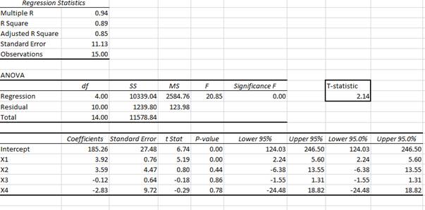
Use the summary output to find the estimated regression equation as follows:
(b)
Economic interpretation of each estimated regression coefficients.
(b)
Explanation of Solution
Interpretation of estimated slope (b) coefficient:
For a given level of total no. of rooms, age and attached garage, an additional 100 ft2 will lead to rise in selling
For a given level of size, age and attached garage, an additional room will lead to rise in selling price by 3.59×$1000 = $3,590.
For a given level of size, total no. of rooms and attached garage, an additional year of age will lead to fall in selling price by 0.12×$1000 = $120.
For a given level of size, total no. of rooms and age, an additional garage will lead to fall in selling price by 2.83×$1000 = $2,830.
(c)
Statistical significance of the independent variables at 0.05 level.
(c)
Explanation of Solution
Conduct the t-test to know the statistical significance of the independent variables X1, X2, X3 and X4. The test statistic can be calculated using following formula:
The t-statistic follows t-distribution with n-1 degrees of freedom.
For variable X1, t-test is conducted as follows:
According to the summary output, the t-statistic for X1 variable is equal to 5.19.
At 5% significance level and 15-1= 14 degrees of freedom, the critical value is equal to 2.145.
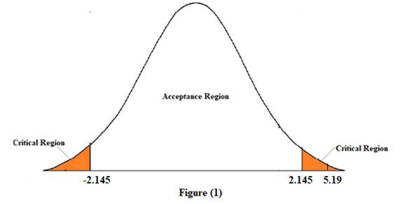
In figure (1), since the calculated t-statistic lies in the critical region. Therefore, we reject the null hypothesis. This means that the variable X1is statistically significant.
For variable X2, t-test is conducted as follows:
According to the summary output, the t-statistic for X2 variable is equal to 0.80.
At 5% significance level and 15-1= 14 degrees of freedom, the critical value is equal to 2.145.
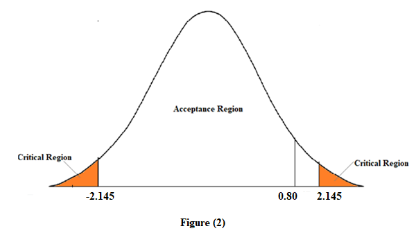
In figure (2), since the calculated t-statistic lies in the acceptance region. Therefore, we accept the null hypothesis. This means that the variable X2is not statistically significant.
For variable X3, t-test is conducted as follows:
According to the summary output, the t-statistic for X3 variable is equal to -0.18.
At 5% significance level and 15-1= 14 degrees of freedom, the critical value is equal to 2.145.
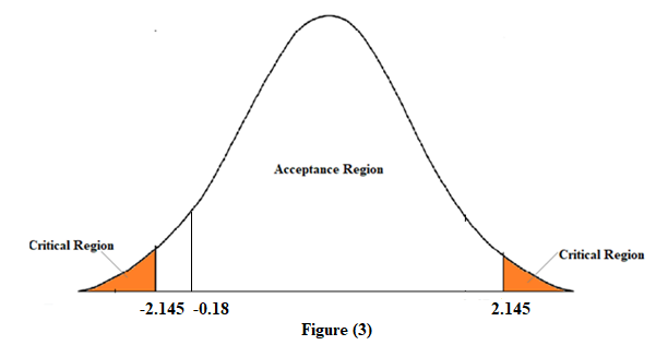
In figure (3), since the calculated t-statistic lies in the acceptance region. Therefore, we accept the null hypothesis. This means that the variable X3is not statistically significant.
For variable X4, t-test is conducted as follows:
According to the summary output, the t-statistic for X4 variable is equal to -0.29.
At 5% significance level and 15-1= 14 degrees of freedom, the critical value is equal to 2.145.
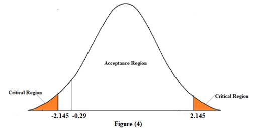
In figure (4), since the calculated t-statistic lies in the acceptance region. Therefore, we accept the null hypothesis. This means that the variable X4is not statistically significant.
(d)
Proportion of total variation in selling price explained by regression model.
(d)
Explanation of Solution
The coefficient of determination measures the proportion of variance predicted by the independent variable in the dependent variable. It is denoted as R2.
According to the summary output, the value of R2 is equal to 0.89. This means that the regression equation predicts 89% of the variance in selling price.
(e)
Overall explanatory power of model by performing F-test at 5 percent level of significance.
(e)
Explanation of Solution
The value of F-statistic is given as 20.85. And the critical value at 0.05 significance level is equal to 0.00.
Since, F-statistic is greater than the critical value. Thus, the overall model is statistically significant.
(f)
95 percent prediction interval for selling price of a 15-year-old house having 1,800 sq. ft., 7 rooms, and an attached garage.
(f)
Explanation of Solution
The confidence interval of a multiple linear regression model can be calculated using following formula:
Here,
y is estimated selling price based on the given values of independent variables
t is critical t value or t-statistic
s.e is multiple standard error of the estimate
The estimated selling price based on the given values of independent variables can be calculated using the estimated regression equation as follows:
According to the regression statistics in the summary output t-statistic and value of multiple standard error of the estimate is equal to 2.14 and 11.13.
Plug the values in the above confidence interval formula as follows:
Thus, an approximate 95% prediction interval for the selling price of a house having an area of a 15-year-old having 1,800 sq. ft., 7 rooms, and an attached garage range from 7291.24 to 7243.60.
Want to see more full solutions like this?
Chapter 4 Solutions
Bundle: Managerial Economics: Applications, Strategies And Tactics, 14th + Mindtap Economics, 1 Term (6 Months) Printed Access Card

- In regression analysis, a common metric used in assessing the quality of the model being used to fit the data is known as the R-squared coefficient. Explain the R-squared coefficient. What is the difference between the R-squared and adjusted R-squared coefficients?arrow_forwardWhich of the following is a consequence of severe multicollinearity in a regression model? A. High standard errors for the estimated coefficientsB. Lower standard errors for the estimated coefficientsC. The OLS estimator becomes biasedD. The dependent variable becomes constantarrow_forwardWhich of the following are plausible approaches to dealing with a model that exhibits heteroscredasticity? i) Take logarithms of each of the variables ii) Use suitably modified standart errors iii) Use generalised least squares procedure iv) Add lagged values of the variables to the regression equation Answers: a- (i), (ii), (iii) and (iv) b- (ii) and (iv) c- (i) and (iii) d- (i), (ii) and (iii) What is the answer?arrow_forward
- Suppose that an economist has been able to gather data on the relationship between demand and price for a particular product. After analyzing scatterplots and using economic theory, the economist decides to estimate an equation of the form Q= aPb, where Q is quantity demanded and P is price. An appropriate regression analysis is then performed, and the estimated parameters turn out to be a = 1000 and b = - 1.3. Now consider two scenarios: (1) the price increases from $10 to $12.50; (2) the price increases from $20 to $25. a. Do you predict the percentage decrease in demand to be the same in scenario 1 as in scenario 2? Why or why not? b. What is the predicted percentage decrease in demand in scenario 1? What about scenario 2? Be as exact as possible.arrow_forwardThe overall significance of an estimated multiple regression model is tested by using _____. Select one: a. F-test b. t-test c. χ^2-test d. None of the abovearrow_forwardThe controller of Chittenango Chain Company believes that the identification of the variable and fixed components of the firm’s costs will enable the firm to make better planning and control decisions. Among the costs the controller is concerned about is the behavior of indirect-materials cost. She believes there is a correlation between machine hours and the amount of indirect materials used.A member of the controller’s staff has suggested that least-squares regression be used to determine the cost behavior of indirect materials. The regression equation shown below was developed from 40 pairs of observations.S = $200 + $9H where S = Total monthly cost of indirect materials H = Machine hours per month The estimated cost of indirect materials if 900 machine hours are to be used during a month is $8,300 (Assume that 900 falls within the relevant range for this cost equation.) The high and low activity levels during the past four years, as measured by machine hours, occurred…arrow_forward
- ABC, Inc., sells tea products to various customers. In recent years, profits have been declining. The CFO of the company investigated the reasons for the profit decline and performed regression analysis for sales and costs. She determined that sales depend on product price, delivery speed, customer services, and marketing expenses. She also determined that total costs consist of variable costs of $25 per unit and fixed costs of $56,000. Marketing expenses have a coefficient of determination of 75% related sales. List two advantages and two limitations of regression analysis.arrow_forwardAs the number of relevant independent variables in a regression increases, the R-squared of a regression Select one: a. exhibits greater heteroskedasticity b. increases c. decreases d. stays constantarrow_forwardThe 2008 sales and profits of seven companies were given as follows Firm Sales ($ Billions) Profit ($ Billions) Fiat 5.7 0.27 Honda 6.7 0.12 BP 0.2 0.01 Toyota 0.6 0.04 Apple 3.8 0.05 IBM 12.5 0.46 Phillips 0.5 0.02 The estimated value for the company’s Profit can be estimated using the equation; Y ̂i = α ̂ + β ̂Xi……………………………………………………………………Eqn.1 Where; Y = Companies Profit X = Companies Sales α ̂ and β ̂ are estimated parameters in the model Calculate the sample regression line, where profit is the dependent variable (Y) and sales is the independent variable (X)arrow_forward
- Addition of explanatory variables in a regression model increases the value of _____. Select one: a. explained sum of squares (ESS) b. residual sum of squares (RSS) c. total sum of squares (TSS) d. Both TSS and ESSarrow_forwardXYZ company is interested in quantifying the impact of consumer promotions on the sales of its packaged food product. XYZ has historical data on the following variables for 38 weeks: • Sales: Weekly sales volume in thousands of units.• Prom: Weekly spending on consumer promotions in thousands of Dollars" "A regression analysis was applied to XYZ historical dataset. The dependent variable is weekly Sales and the independent variables are weekly Prom and weekly Lagged Prom (i.e., last week Prom). This is a summary of the regression output:Sales = 0.80 + 1.20*Prom - 0.40*Lag(Prom) • R-squared=0.85• F-Statistic=23.83• p-value=0.001 (for the overall regression)•All regression coefficients are statistically significant at the 5% level." A. What will be the predicted sales volume ? B. What is the gross margin of this net volume impact due to $1000 spending per week on consumer promotions, if brand makes $2.20 gross margin per unit . C. What is the ROI of this promotion? D. What is predicted…arrow_forwardThe assumption that the error terms in a regression model follow the normal distribution with zero mean and constant variance is required Select one: Estimation of the regression model using OLS method Point estimation of the parameters Hypothesis testing and inference Inference One of the assumption of CLRM is that the number of observations in the sample must me greater the number of Select one: Dependent and independent variable Dependent Variable Regressor Regressands Information about numerical values of variables from period to period is Select one: Time series data Pooled data Panel data Cross section data Multicollinearity is essentially a Select one: Sample phenomenon or population phenomenon sample phenomenon Sample phenomenon and population phenomenon Population phenomenon The larger the standard error of the estimator, the greater is the uncertainty of estimating the true value of the unknown parameters. This statement is Select one: True Falsearrow_forward
 Managerial Economics: Applications, Strategies an...EconomicsISBN:9781305506381Author:James R. McGuigan, R. Charles Moyer, Frederick H.deB. HarrisPublisher:Cengage Learning