
Whether there was a statistically significant difference in the average speeds, the mean speed, standard deviation, 85th percentile speed and percentage of traffic exceeding the posted speed limit of 30 mi/h.
Answer to Problem 9P
Significant reduction
Explanation of Solution
Given:
Significance level of
Formula used:
S is standard deviation
N is number of observations
Spis square root of the pooled variance
S1 and S2 are standard deviations of the populations
T is the test static
Calculation:
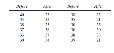
Before an increase in speed enforcement activities:
The speed ranges from 28 to 40 mi/hgiving a speed range of 12. For five classes, the range per class is 2.4mi/h. A frequency distribution table can then be prepared, as shown below, in which the speed classes are listed in column 1 and the mid-values are in column 2. The number of observationsfor each class is listed in column 3, the cumulative percentages of all observations arelisted in column 6.
| 1 | 2 | 3 | 4 | 5 | 6 | 7 |
| Speed class (mi/h) | Class mid-value | Class frequency, | | Percentage of class frequency | Cumulative percentage of class frequency | |
| 28-30 | 29 | 4 | 116 | 13 | 13 | 139.24 |
| 31-33 | 32 | 5 | 160 | 17 | 30 | 42.05 |
| 34-36 | 35 | 12 | 420 | 40 | 70 | 0.12 |
| 37-39 | 38 | 6 | 228 | 20 | 90 | 57.66 |
| 40-42 | 41 | 3 | 123 | 10 | 100 | 111.63 |
| Total | 30 | 1047 | 350.7 |
Determine the arithmetic mean speed:
Determine the standard deviation:
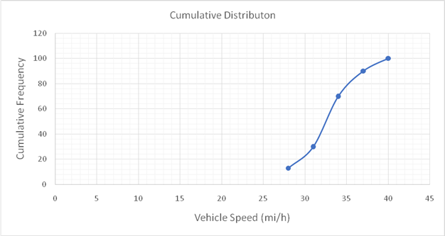
The 85th-percentile speed is obtained from the cumulative frequency distribution curve as 36 mi/h.
The percentage of traffic exceeding the posted speed limit of 30 mi/h is 76 %.
Below given figure shows the cumulative frequency distribution curve for the data given. In this case, the cumulative percentages in column 6 of the above Table are plotted against the upper limit of each corresponding speed class. This curve, therefore, gives the percentage of vehicles that are traveling at or below a given speed.
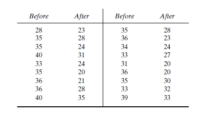
After an increase in speed enforcement activities:
The speed ranges from 20 to 37 mi/h giving a speed range of 17. For six classes, the range per class is 2.83 mi/h. A frequency distribution table can then be prepared, as shown below in which the speed classes are listed in column 1 and the mid-values are in column 2. The number of observations for each class is listed in column 3, the cumulative percentages of all observations are listed in column 6.
| 1 | 2 | 3 | 4 | 5 | 6 | 7 |
| Speed class (mi/h) | Class mid-value | Class frequency, | | Percentage of class frequency | Cumulative percentage of class frequency | |
| 20-22 | 21 | 6 | 126 | 20 | 20 | 253.5 |
| 23-25 | 24 | 8 | 192 | 27 | 47 | 98 |
| 26-28 | 27 | 4 | 108 | 13 | 60 | 1 |
| 29-31 | 30 | 3 | 90 | 10 | 70 | 18.75 |
| 32-34 | 33 | 5 | 165 | 17 | 87 | 151.25 |
| 35-37 | 36 | 4 | 144 | 13 | 100 | 289 |
| Total | 30 | 825 | 811.5 |
Determine the arithmetic mean speed:
Determine the standard deviation:
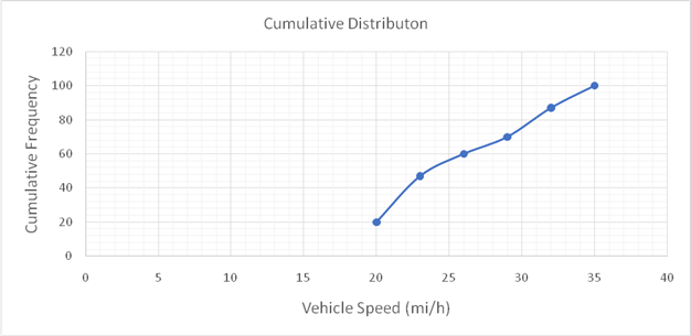
Below given figure shows the cumulative frequency distribution curve for the data given. In this case, the cumulative percentages in column 6 of the above Table are plotted against the upper limit of each corresponding speed class. This curve, therefore, gives the percentage of vehicles that are traveling at or below a given speed.
The 85th-percentile speed is obtained from the cumulative frequency distribution curve as 31.5 mi/h.
The percentage of traffic exceeding the posted speed limit of 30 mi/h is 24 %.
Determine square root of the pooled variance:
Compute test static T:
Determine whether
From Appendix A, theoretical
Since
Conclusion:
The increase in speed enforcement activities has resulted in a significant reduction in the mean speed on the street at a significance level of 0.05. The mean speeds before and after increase in speed enforcement activities are 35.1 and 27.47 mi/h respectively. The standard deviations are 3.5 and 5.3 mi/h respectively. The 85th percentile speeds are 36 mi/h and 31.5 mi/h and percentages of traffic exceeding the posted speed limit of 30 mi/h are 76 % and 24 %.
Want to see more full solutions like this?
Chapter 4 Solutions
TRAFFIC AND HIGHWAY ENG (LL) + WEBASSIG

- An engineer, wishing to determine the travel time and average speed along a section of an urban highway as part of an annual trend analysis on traffic operations, conducted a travel time study using the floating-car technique. He carried out 10 runs and obtained a standard deviation of ±3.4 mi/hin the speeds obtained. If a 5 percent significance level is assumed, is the number of test runs adequate?arrow_forwardThe time between arrivals of vehicles at a particular intersection follows an exponential probability distribution with a mean of 12 seconds. A. Write down the p.d.f. B. What is the probability the time between vehicle arrivals is 12 seconds or less? C. What is the probability there will be 30 or more seconds between arriving vehicles?arrow_forwardFor a spot speed study in which 100 observations were obtained, the mean speed was 52 km/h and the standard deviation was 4.6 km/h. (BO0K: Traffic % Highway engineering, N. Gruber SI unit) What is the margin of error on the estimate of true mean speed obtained from this sample? What is a reasonable estimate of the 85th percentile speed based on the information available?arrow_forward
- At an impaired driver checkpoint, the time required to conduct the impairment test varies (exponentially distributed) depending on the compliance of the driver, but takes 60 seconds on average. If an average of 30 vehicles per hour arrive (according to a Poisson distribution) at the checkpoint, determine the average time spent in the system.arrow_forwardengineer wishing to determine the travel time and average speed along a section of an urban highway as part annual trends analysis on traffic operations conducted a travel time study using the floating -car technique .He carried out 10 runs and obtained a standard deviation of +-3 mi/h in the speeds obtained .if 5% significance level is assumed is the number of test runs adequate?arrow_forwardThe arrival of vehicles at a specified roadway location is Poisson distributed. The flow count shows 540 veh/hr at this roadway location. - What is the probability that headway between successive vehicles will be less than 6 seconds? - What is the probability that headway between successive vehicles will be greater than than 12 seconds? - What is the probability that headway between successive vehicles will be between 6 and 12 seconds? - Draw the probability density function of the exponential distribution and show the key items in the graph. - Draw the cumulative distribution of the exponential distribution and show the key items in the graph.arrow_forward
- A spot speed study was conducted on a freeway on which the mean speed and standard deviation were found to be 72.4 km/h and 5.4 km/h, respectively. What is the range of values that would be expected to contain the middle 95% speeds 1 what is top and the lowest rangearrow_forwardExponential distribution. The time between arrivals of vehicles at a particular intersection follows an exponential probability distribution with a mean of 10 seconds. What is the probability of 30 or more seconds between vehicle arrivals?arrow_forwardA researcher was observing traffic along one lane of a rural highway. During a 1 minute time interval, ten vehicles were observed travelling 65, 64, 71, 66, 58, 72, 69, 66, 55 and 62 mph. Using these spot speeds, calculate the space mean speed (mph). Provide your answer to the nearest tenth of a mph.arrow_forward
- The time between arrivals of vehicles at particular intersection follows an exponential probability distribution with a mean of 15 seconds. What is the probability that the arrival time between vehicles is 9 seconds or less?arrow_forwardAn engineer, wishing to determine the travel time and average speed along a sectionof an urban highway as part of an annual trend analysis on traffic operations, conducteda travel time study using the floating-car technique. He carried out 10 runs andobtained a standard deviation of ±3 mi/h in the speeds obtained. If a 5% significancelevel is assumed, is the number of test runs adequate?arrow_forward
 Traffic and Highway EngineeringCivil EngineeringISBN:9781305156241Author:Garber, Nicholas J.Publisher:Cengage Learning