Problems 51–58 refer to the following slope fields: Figure for 51–58 58. Use a graphing calculator to graph y = Ce x − 1 for C = −2. −1, 1. and 2, for −5 ≤ x ≤ 5, −5 ≤ y ≤ 5, all in the same viewing window. Observe how the solution curves go with the flow of the tangent line segments in the corresponding slope field shown in Figure A or Figure B.
Problems 51–58 refer to the following slope fields: Figure for 51–58 58. Use a graphing calculator to graph y = Ce x − 1 for C = −2. −1, 1. and 2, for −5 ≤ x ≤ 5, −5 ≤ y ≤ 5, all in the same viewing window. Observe how the solution curves go with the flow of the tangent line segments in the corresponding slope field shown in Figure A or Figure B.
Solution Summary: The author explains how to draw the graph of the general solution of y=Cex-1 of differential equation for C=-2,1 and 2.
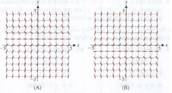
Problems 51–58 refer to the following slope fields:
Figure for 51–58
58. Use a graphing calculator to graph y = Cex − 1 for C = −2. −1, 1. and 2, for −5 ≤ x ≤ 5, −5 ≤ y ≤ 5, all in the same viewing window. Observe how the solution curves go with the flow of the tangent line segments in the corresponding slope field shown in Figure A or Figure B.
In Problems 11–18, match each graph to its function.A. Constant function B. Identity function C. Square function D. Cube functionE. Square root function F. Reciprocal function G. Absolute value function H. Cube root function
In Problems 101–104, graph each function. Based on the graph, state the domain and the range, and find any intercepts.
In Problems 37–44, find the midpoint of the line segment joining the points P1 and P2 .
Chapter 5 Solutions
Calculus for Business, Economics, Life Sciences, and Social Sciences - Boston U.
Using & Understanding Mathematics: A Quantitative Reasoning Approach (7th Edition)
Knowledge Booster
Learn more about
Need a deep-dive on the concept behind this application? Look no further. Learn more about this topic, subject and related others by exploring similar questions and additional content below.
 58. Use a graphing calculator to graph y = Cex − 1 for C = −2. −1, 1. and 2, for −5 ≤ x ≤ 5, −5 ≤ y ≤ 5, all in the same viewing window. Observe how the solution curves go with the flow of the tangent line segments in the corresponding slope field shown in Figure A or Figure B.


 Algebra & Trigonometry with Analytic GeometryAlgebraISBN:9781133382119Author:SwokowskiPublisher:Cengage
 Glencoe Algebra 1, Student Edition, 9780079039897...AlgebraISBN:9780079039897Author:CarterPublisher:McGraw Hill
 Trigonometry (MindTap Course List)TrigonometryISBN:9781305652224Author:Charles P. McKeague, Mark D. TurnerPublisher:Cengage Learning
 Calculus For The Life SciencesCalculusISBN:9780321964038Author:GREENWELL, Raymond N., RITCHEY, Nathan P., Lial, Margaret L.Publisher:Pearson Addison Wesley,