
(a)
Interpretation:
Poles and zeros of the given transfer function are to be plotted on a complex plane.
Concept introduction:
For any transfer function
For any transfer function
Answer to Problem 6.1E
The plot of the poles and zeros of the given transfer function on the complex plane as:

Explanation of Solution
Given information:
The given transfer function is:
For the given transfer function, the numerator polynomial is:
To calculate the zeros of the given transfer function, equation this polynomial to zero and calculate its roots using MATLAB commands as shown below:

The compiler will generate its roots as:
These are the zeros of the given transfer function.
For the given transfer function, the denominator polynomial is:
To calculate the poles of the given transfer function, equation this polynomial to zero and calculate its roots using MATLAB commands as shown below:

The compiler will generate its roots as:
These are the poles of the given transfer function.
Now, plot these poles and zeros on the complex plane as:

(b)
Interpretation:
The conclusion regarding the output modes for any input changes is to be determined from the location of poles in the complex plane.
Concept introduction:
For any transfer function
For any transfer function
The complex plane is divided into two halves: Left Half Plane and Right Half Plane. The Left Half Plane represents the stable region and the Right Half Plane represents the unstable region.
Answer to Problem 6.1E
Any change in the input of the process will lead to the unbounded and unstable output as two of the poles of the given transfer function lie in the Right Half Plane.
Explanation of Solution
Given information:
The given transfer function is:
From part (a), the plot of poles and zeros of the given polynomial is:
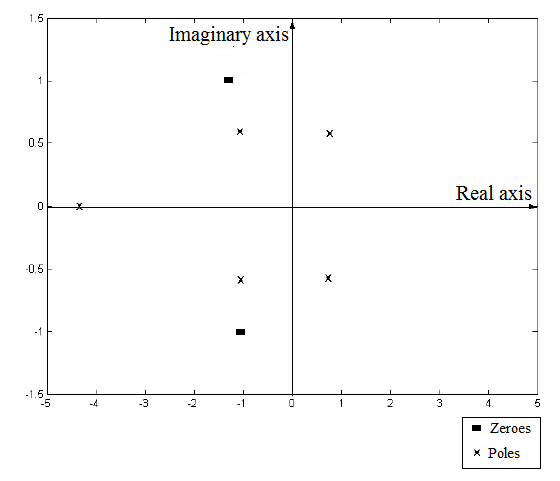
From this plot, two of the poles lie in the Right Half Plane of the complex plane. This makes the process output unstable. Therefore, any change in the input of the process will lead to unbounded and unstable output.
(c)
Interpretation:
The output response for the unit step change in the input for the given transfer function is to be plotted and its correctness to the analysis of the output mode made in part (b) is to be done.
Concept introduction:
For any transfer function
For any transfer function
The complex plane is divided into two halves: Left Half Plane and Right Half Plane. The Left Half Plane represents the stable region and the Right Half Plane represents the unstable region.
Answer to Problem 6.1E
The response of the given transfer function for a unit step change in the input is:
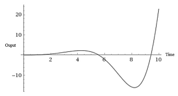
The output response of the process is unstable and unbounded for the step-change in the input which agrees with the analysis done in part (b).
Explanation of Solution
Given information:
The given transfer function is:
For a unit step change in the input, the value of
Substitute this value of
The plot of the response of this transfer function using the online tool will be:

In part (b), it was analyzed that the poles pair in the Right Half Plane makes the system output unbounded and stable. From the response plot shown above, this analysis is correct as the output response of the process is unstable and unbounded for the step-change in the input.
Want to see more full solutions like this?
Chapter 6 Solutions
EBK PROCESS DYNAMICS+CONTROL

 Introduction to Chemical Engineering Thermodynami...Chemical EngineeringISBN:9781259696527Author:J.M. Smith Termodinamica en ingenieria quimica, Hendrick C Van Ness, Michael Abbott, Mark SwihartPublisher:McGraw-Hill Education
 Elementary Principles of Chemical Processes, Bind...Chemical EngineeringISBN:9781118431221Author:Richard M. Felder, Ronald W. Rousseau, Lisa G. BullardPublisher:WILEY
 Elements of Chemical Reaction Engineering (5th Ed...Chemical EngineeringISBN:9780133887518Author:H. Scott FoglerPublisher:Prentice Hall
 Industrial Plastics: Theory and ApplicationsChemical EngineeringISBN:9781285061238Author:Lokensgard, ErikPublisher:Delmar Cengage Learning
 Unit Operations of Chemical EngineeringChemical EngineeringISBN:9780072848236Author:Warren McCabe, Julian C. Smith, Peter HarriottPublisher:McGraw-Hill Companies, The