Concept explainers
Videos
John can take either of two routes (A or B) to LAX airport. At midday on a typical Wednesday the travel time on either route is
a.
Find the better route for John to reach at the airport in 54 minutes to pick up his spouse.
Answer to Problem 91CE
The better route for John to reach at the airport in 54 minutes to pick up his spouse is route A.
Explanation of Solution
Calculation:
It is given that the time on route A follows normal distribution with mean of 54 minutes, standard deviation of 6 minutes and the time on route B follows normal distribution with mean of 60 minutes, standard deviation of 3 minutes.
Normal distribution:
A continuous random variable X is said to follow normal distribution if the probability density function of X is,
Assume that the random variable X denotes the time to reach airport.
For route A:
It is given that
Now, the probability to reach at the airport in 54 minutes using route A, implies that
Probability value:
Software procedure:
Step-by-step software procedure to obtain probability value using EXCEL is as follows:
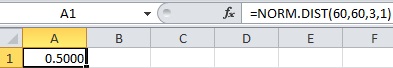
- Open an EXCEL file.
- In cell A1, enter the formula “=NORM.DIST(54,54,6,1)”.
- Output using EXCEL software is given below:
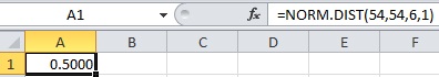
Therefore,
Thus, the probability to reach at the airport in 54 minutes using route A is 0.5.
For route B:
It is given that
Now, the probability to reach at the airport in 54 minutes using route B, implies that
Probability value:
Software procedure:
Step-by-step software procedure to obtain probability value using EXCEL is as follows:
- Open an EXCEL file.
- In cell A1, enter the formula “=NORM.DIST(54,60,3,1)”.
- Output using EXCEL software is given below:
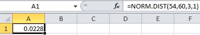
Therefore,
Thus, the probability to reach at the airport in 54 minutes using route B is 0.0228.
Therefore, there is more chance to reach airport by route A than by route B.
Thus, the better route for John to reach at the airport in 54 minutes to pick up his spouse is route A.
b.
Find the better route for John to reach at the airport in 66 minutes to pick up his spouse.
Answer to Problem 91CE
The better route for John to reach at the airport in 60 minutes to pick up his spouse is route A.
Explanation of Solution
Calculation:
For route A:
It is given that
Now, the probability to reach at the airport in 66 minutes using route A, implies that
Probability value:
Software procedure:
Step-by-step software procedure to obtain probability value using EXCEL is as follows:
- Open an EXCEL file.
- In cell A1, enter the formula “=NORM.DIST(60,54,6,1)”.
- Output using EXCEL software is given below:
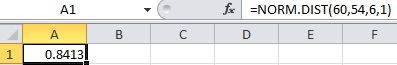
Therefore,
Thus, the probability to reach at the airport in 60 minutes using route A is 0.8413.
For route B:
It is given that
Now, the probability to reach at the airport in 60 minutes using route B, implies that
Probability value:
Software procedure:
Step-by-step software procedure to obtain probability value using EXCEL is as follows:
- Open an EXCEL file.
- In cell A1, enter the formula “=NORM.DIST(60,60,3,1)”.
- Output using EXCEL software is given below:
Therefore,
Thus, the probability to reach at the airport in 60 minutes using route B is 0.5.
Therefore, there is more chance to reach airport by route A than by route B.
Thus, the better route for John to reach at the airport in 60 minutes to pick up his spouse is route A.
c.
Find the better route for John to reach at the airport in 60 minutes to pick up his spouse.
Answer to Problem 91CE
The better route for John to reach at the airport in 66 minutes to pick up his spouse is route B.
Explanation of Solution
Calculation:
Coefficient of variation:
Coefficient of variation for a random variable X is defined as,
It is better to use a random variable with lower CV.
For route A:
It is given that
Now, the probability to reach at the airport in 66 minutes using route A, implies that
Probability value:
Software procedure:
Step-by-step software procedure to obtain probability value using EXCEL is as follows:
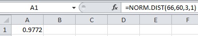
- Open an EXCEL file.
- In cell A1, enter the formula “=NORM.DIST(66,54,6,1)”.
- Output using EXCEL software is given below:
Therefore,
Thus, the probability to reach at the airport in 66 minutes using route A is 0.9972.
The CV for route A is,
For route B:
It is given that
Now, the probability to reach at the airport in 66 minutes using route B, implies that
Probability value:
Software procedure:
Step-by-step software procedure to obtain probability value using EXCEL is as follows:
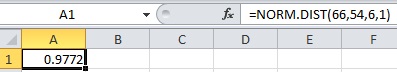
- Open an EXCEL file.
- In cell A1, enter the formula “=NORM.DIST(66,60,3,1)”.
- Output using EXCEL software is given below:
Therefore,
Thus, the probability to reach at the airport in 66 minutes using route B is 0.9972.
The CV for route B is,
Therefore, there is same chance to reach airport by route A and route B.
Now, the coefficient of variation for route B is less than route A.
Thus, the better route for John to reach at the airport in 66 minutes to pick up his spouse is route B.
Want to see more full solutions like this?
Chapter 7 Solutions
Applied Statistics in Business and Economics


- Experiment 1: An agronomist wanted to compare the yield of three different varieties of rice (A, B, C). So, within a field, he randomly assigned each variety to five plots. The yield[s] in pounds per acre were recorded for each plot. Go back to the original experiment in (1) where we are only interested in variety, not fertilizer. The agronomist realized that he wanted his results to apply over a range of soil conditions. So, he decided to conduct the experiment on 4 different locations (subdivisions) in a field so that the elevation and type of soil vary. He planted each variety on one plot within each subdivision of the field. Again, the yield[s] in pounds per acre were recorded for each plot. (d) What are the experimental units in the study? How many are there in total? (e) What is the name of the design of this experiment? (Single factor, two-factor, block) (f) Outline the design of the experiment.arrow_forwardExperiment 1: An agronomist wanted to compare the yield of three different varieties of rice (A, B, C). So, within a field, he randomly assigned each variety to five plots. The yield[s] in pounds per acre were recorded for each plot. Go back to the original experiment in (1) where we are only interested in variety, not fertilizer. The agronomist realized that he wanted his results to apply over a range of soil conditions. So, he decided to conduct the experiment on 4 different locations (subdivisions) in a field so that the elevation and type of soil vary. He planted each variety on one plot within each subdivision of the field. Again, the yield[s] in pounds per acre were recorded for each plot. (a) What is the response in the study? (b) What is the factor in the study? What are the factor levels? (c) What are the treatments? What are the blocks, if any?arrow_forwardA well-known maker of jams and jellies packages its jams in jars labeled "~250 milliliters." The process used to fill the jars is known to dispense an amount of jam that is a Normally distributed variable µ = 252 milliliters and σ = 0.9 milliliters. What proportion of jars will be filled with what the label claims is 250 milliliters?arrow_forward
- An industrial concern has experimented with several different mixtures of the fourcomponents—magnesium, sodium nitrate, strontium nitrate, and a binder—that comprise arocket propellant. The company has found that two mixtures, in particular, give higher flare illumination values than the others. Mixture 1 consists of a blend composed of the proportions.40, .10, .42, and .08, respectively, for the four components of the mixture; mixture 2 consists ofa blend using the proportions .60, .25, .10, and .05. Twenty different blends (10 of each mixture)are prepared and tested to obtain the flare-illumination values. These data appear here (in unitsof 1,000 candles).Mixture 1 185 192 201 215 170 190 175 172 198 202Mixture 2 221 210 215 202 204 196 225 230 214 217a. Plot the sample data. Which test(s) could be used to compare the meanillumination values for the two mixtures?b. Give the level of significance of the test and interpret your findingsarrow_forwardThe scatterplot of these two variables reveals a potential outlying month when the average temperature is about 53◦F and average crawling age is about 28.5 weeks. (a) Does this point have high leverage? (b) Is it an influential point?arrow_forwardProfessor Cambridge collected data from each of his 1st year Chemistry student. If the population if Professor Cambridge’s Chemistry students (all students in the data set) is it possible to calculate the parameters? Or it is limited only to statistics? Why do you think so? If the population involves both the junior and senior students, and the dataset is the sample from that population, is it possible to calculate the parameters for that population? Or is it limited to statistics? Why do you think so?arrow_forward
- The least-squares regression equation is y=620.6x+16,624 where y is the median income and x is the percentage of 25 years and older with at least a bachelor's degree in the region. The scatter diagram indicates a linear relation between the two variables with a correlation coefficient of 0.7004. In a particular region, 28.3 percent of adults 25 years and older have at least a bachelor's degree. The median income in this region is $37,389. Is this income higher than what you would expect? Why?arrow_forwardThe personnel department of a large corporation gives two aptitude tests to job applicants. From many years’ experience, the company has found that a person’s score for the first test, Y1, is normally distributed with μ1 = 50 and σ1 = 10. The scores for the second test, Y2, are normally distributed with μ2 = 100 and σ2 = 20. A composite score, Y, is assigned to each applicant, where Y = 3Y1 + 2Y2. To avoid unnecessary paperwork, the company automatically rejects any applicant whose composite score is below 375. If six individuals submit résumés, what are the chances that fewer than half will fail the screening tests? Hint: Use the fact that the sum of two independent normal random variables is also a normal random variable.arrow_forwardThe least-squares regression equation is y=784.6x+12,431 where y is the median income and x is the percentage of 25 years and older with at least a bachelor's degree in the region. The scatter diagram indicates a linear relation between the two variables with a correlation coefficient of 0.7962. In a particular region, 26.5 percent of adults 25 years and older have at least a bachelor's degree. The median income in this region is $29,889. Is this income higher or lower than what you would expect? Why?arrow_forward
- The least-squares regression equation is y=647.8x+17,858 where y is the median income and x is the percentage of 25 years and older with at least a bachelor's degree in the region. The scatter diagram indicates a linear relation between the two variables with a correlation coefficient of 0.7507. predict the median income of a region in which 20% of adults 25 years and older have at least a bachelor's degree. Round to the nearest dollar as needed.arrow_forwardIn the Chernobyl nuclear accident it is estimated that 30,000 people received an average dose of 45 REM. For this population, using the linear hypothesis, how many "normal" deaths from cancer are expected and how many additional deaths from the radiation of the accident? Group of answer choices 500 normal, 6000 additional 1000 normal, 4000 additional 2000 normal, 3000 additional 4000 normal, 1000 additional 6000 normal, 500 additionalarrow_forwardWhen 20 employees were first hired in 2011 for a creative engineering firm, Company A, the starting annual salary was $35,000. A competing creative engineering firm, Company B, had the same starting salary for 20 employees hired the same year. In 2016, data was collected on the annual salaries of the same employees at each of the two companyies. This data is displayed in the box plot shown. Part A: Compare the annual salary distributions and what are the pros and cons of working at each company? Explain using what you found in Part Aarrow_forward
 Linear Algebra: A Modern IntroductionAlgebraISBN:9781285463247Author:David PoolePublisher:Cengage Learning