Travels with My Ant: The Curtate and Prolate Cycloids Earlier in this section, we looked at the parametric equations for a cycloid, which is the path a point on the edge of a wheel traces as the wheel rolls along a straight path. In this project we look at two different variations of the cycloid, called the curtate and prolate cycloids. First, let’s revisit the derivation of the parametric equations for a cycloid. Recall that we considered a tenacious ant trying to get home by hanging onto the edge of a bicycle tire. We have assumed the ant climbed onto the tire at the very edge, where the tire touches the ground. As the wheel rolls, the ant moves with the edge of the tire (Figure 7.13). As we have discussed, we have a lot of ?exibility when parameterizing a curve. In this case we let our parameter t represent the angle the tire has rotated through. Looking at Figure 7.13, we see that after the tire has rotated through an angle of t, the position of the center of the wheel, C = ( x C , y C ) , is given by x C = a t and y C = a . Furthermore, letting A = ( x A , y A ) denote the position of the ant, we note that x C − x A = a sin t and y C − y A = a cos t . Then x A = x C − a sin t = a t − a sin t = a ( t − sin t ) y A = y C − a cos t = a − a cos t = a ( 1 − cos t ) . Figure 7.13 (a) The ant clings to the edge of the bicycle tire as the tire rolls along the ground. (b) Using geometry to determine the position of the ant after the tire has rotated through an angle of t. Note that these are the same parametric representations we had before, but we have now assigned a physical meaning to the parametric variable t. After a while the ant is getting dizzy from going round and round on the edge of the tire. So he climbs up one of the spokes toward the center of the wheel. By climbing toward the center of the wheel, the ant has changed his path of motion. The new path has less up—and-down motion and is called a curtate cycloid (Figure 7.14). As shown in the figure, we let b denote the distance along the spoke from the center of the wheel to the ant. As before, we let t represent the angle the tire has rotated through. Additionally, we let C = ( x C , y C ) represent the position of the center of the wheel and A = ( x A , y A ) represent the position of the ant. Figure 7.14 (a) The ant climbs up one of the spokes toward the center of the wheel. (b) The ant’s path of motion after he climbs closer to the center of the wheel. This is called a curtate cycloid. (c) The new setup, now that the ant has moved closer to the center of the wheel. 5. What do you notice about your answer to part 3 and your answer to part 4? Notice that the ant is actually traveling backward at times (the “loops” in the graph), even though the train continues to move forward. He is probably going to be real1y dizzy by the time he gets home!
Travels with My Ant: The Curtate and Prolate Cycloids Earlier in this section, we looked at the parametric equations for a cycloid, which is the path a point on the edge of a wheel traces as the wheel rolls along a straight path. In this project we look at two different variations of the cycloid, called the curtate and prolate cycloids. First, let’s revisit the derivation of the parametric equations for a cycloid. Recall that we considered a tenacious ant trying to get home by hanging onto the edge of a bicycle tire. We have assumed the ant climbed onto the tire at the very edge, where the tire touches the ground. As the wheel rolls, the ant moves with the edge of the tire (Figure 7.13). As we have discussed, we have a lot of ?exibility when parameterizing a curve. In this case we let our parameter t represent the angle the tire has rotated through. Looking at Figure 7.13, we see that after the tire has rotated through an angle of t, the position of the center of the wheel, C = ( x C , y C ) , is given by x C = a t and y C = a . Furthermore, letting A = ( x A , y A ) denote the position of the ant, we note that x C − x A = a sin t and y C − y A = a cos t . Then x A = x C − a sin t = a t − a sin t = a ( t − sin t ) y A = y C − a cos t = a − a cos t = a ( 1 − cos t ) . Figure 7.13 (a) The ant clings to the edge of the bicycle tire as the tire rolls along the ground. (b) Using geometry to determine the position of the ant after the tire has rotated through an angle of t. Note that these are the same parametric representations we had before, but we have now assigned a physical meaning to the parametric variable t. After a while the ant is getting dizzy from going round and round on the edge of the tire. So he climbs up one of the spokes toward the center of the wheel. By climbing toward the center of the wheel, the ant has changed his path of motion. The new path has less up—and-down motion and is called a curtate cycloid (Figure 7.14). As shown in the figure, we let b denote the distance along the spoke from the center of the wheel to the ant. As before, we let t represent the angle the tire has rotated through. Additionally, we let C = ( x C , y C ) represent the position of the center of the wheel and A = ( x A , y A ) represent the position of the ant. Figure 7.14 (a) The ant climbs up one of the spokes toward the center of the wheel. (b) The ant’s path of motion after he climbs closer to the center of the wheel. This is called a curtate cycloid. (c) The new setup, now that the ant has moved closer to the center of the wheel. 5. What do you notice about your answer to part 3 and your answer to part 4? Notice that the ant is actually traveling backward at times (the “loops” in the graph), even though the train continues to move forward. He is probably going to be real1y dizzy by the time he gets home!
Travels with My Ant: The Curtate and Prolate Cycloids
Earlier in this section, we looked at the parametric equations for a cycloid, which is the path a point on the edge of a wheel traces as the wheel rolls along a straight path. In this project we look at two different variations of the cycloid, called the curtate and prolate cycloids.
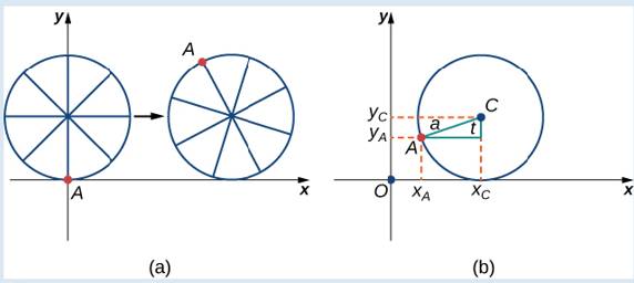
First, let’s revisit the derivation of the parametric equations for a cycloid. Recall that we considered a tenacious ant trying to get home by hanging onto the edge of a bicycle tire. We have assumed the ant climbed onto the tire at the very edge, where the tire touches the ground. As the wheel rolls, the ant moves with the edge of the tire (Figure 7.13).
As we have discussed, we have a lot of ?exibility when parameterizing a curve. In this case we let our parameter t represent the angle the tire has rotated through. Looking at Figure 7.13, we see that after the tire has rotated through an angle of t, the position of the center of the wheel,
C
=
(
x
C
,
y
C
)
, is given by
x
C
=
a
t
and
y
C
=
a
.
Furthermore, letting
A
=
(
x
A
,
y
A
)
denote the position of the ant, we note that
x
C
−
x
A
=
a
sin
t
and
y
C
−
y
A
=
a
cos
t
.
Then
x
A
=
x
C
−
a
sin
t
=
a
t
−
a
sin
t
=
a
(
t
−
sin
t
)
y
A
=
y
C
−
a
cos
t
=
a
−
a
cos
t
=
a
(
1
−
cos
t
)
.
Figure 7.13 (a) The ant clings to the edge of the bicycle tire as the tire rolls along the ground. (b) Using geometry to determine the position of the ant after the tire has rotated through an angle of t.
Note that these are the same parametric representations we had before, but we have now assigned a physical meaning to the parametric variable t.
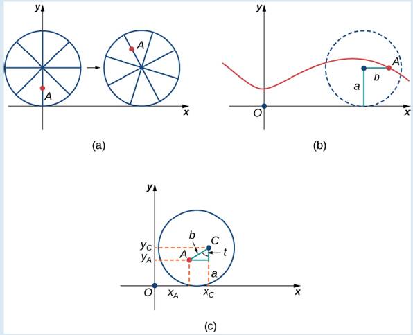
After a while the ant is getting dizzy from going round and round on the edge of the tire. So he climbs up one of the spokes toward the center of the wheel. By climbing toward the center of the wheel, the ant has changed his path of motion. The new path has less up—and-down motion and is called a curtate cycloid (Figure 7.14). As shown in the figure, we let b denote the distance along the spoke from the center of the wheel to the ant. As before, we let t represent the angle the tire has rotated through. Additionally, we let
C
=
(
x
C
,
y
C
)
represent the position of the center of the wheel and
A
=
(
x
A
,
y
A
)
represent the position of the ant.
Figure 7.14 (a) The ant climbs up one of the spokes toward the center of the wheel. (b) The ant’s path of motion after he climbs closer to the center of the wheel. This is called a curtate cycloid. (c) The new setup, now that the ant has moved closer to the center of the wheel.
5. What do you notice about your answer to part 3 and your answer to part 4?
Notice that the ant is actually traveling backward at times (the “loops” in the graph), even though the train continues to move forward. He is probably going to be real1y dizzy by the time he gets home!
Finite Mathematics for Business, Economics, Life Sciences and Social Sciences
Knowledge Booster
Learn more about
Need a deep-dive on the concept behind this application? Look no further. Learn more about this topic, subject and related others by exploring similar questions and additional content below.


 Algebra and Trigonometry (MindTap Course List)AlgebraISBN:9781305071742Author:James Stewart, Lothar Redlin, Saleem WatsonPublisher:Cengage Learning
 Trigonometry (MindTap Course List)TrigonometryISBN:9781337278461Author:Ron LarsonPublisher:Cengage Learning
 Algebra & Trigonometry with Analytic GeometryAlgebraISBN:9781133382119Author:SwokowskiPublisher:Cengage