EBK INTRODUCTION TO PROBABILITY AND STA
14th Edition
ISBN: 8220100445279
Author: BEAVER
Publisher: CENGAGE L
bartleby

Concept explainers

bartleby

Videos

Textbook Question
Book Icon
Chapter 7.5, Problem 7.17E

A population consists of N = 5 numbers: 1, 3, 5, 6, and 7. It can be shown that the mean and standard deviation for this population are μ = 4.4 and σ = 2.15 , respectively.

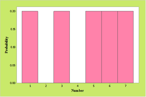
a. Construct a probability histogram for this population.

b. Use the random number table. Table 10 in Appendix I, to select a random sample of size n = 10 with replacement from the population. Calculate the sample mean. x ¯ . Repeat this procedure. calculating the sample mean x ¯ for your second sample.

(HINT: Assign the random digits 0 and 1 to the measurement x = 1 ; assign digits 2 and 3 to the measurement x = 3 , and so on.)

c. To simulate the sampling distribution of x ¯ , we have selected 50 more samples of size n = 10 with replacement, and have calculated the corresponding sample means. Construct a relative frequency histogram for these 50 values of x ¯ . What is the shape of this distribution?

Chapter 7.5, Problem 7.17E, A population consists of N=5 numbers: 1, 3, 5, 6, and 7. It can be shown that the mean and standard

a.

Expert Solution
Check Mark
To determine

To graph: A probability histogram for the data.

Explanation of Solution

Given information:

The given population contain N=5 values such that

  1,3,5,6, and 7 .

The population mean μ=4.4 and the population standard deviation σ=2.15 .

Calculation:

Here there are five numbers without repeating therefore the probability of each number to be equal. Hence the probability for a number is

  15=0.2.

Graph:

In the below histogram height of the bars equal to the probability.

  EBK INTRODUCTION TO PROBABILITY AND STA, Chapter 7.5, Problem 7.17E , additional homework tip  1

b.

Expert Solution
Check Mark
To determine

To find: The two sets of samples of size n=10 using the random number Table 10 in Appendix I and theirmean values.

Answer to Problem 7.17E

The first selected sample is 1, 5, 5, 7, 3, 1, 6, 7, 1, 3 and x¯=3.9 .

The second selected sample is 1, 5, 3, 6, 1, 1, 6, 5, 3, 3 and x¯=3.4 .

Explanation of Solution

Given information:

The random digits 0 and 1 corresponds with the number 1 ; the random digits 2 and 3 corresponds with the number 3 ; the random digits 4 and 5 corresponds with the number 5 ; the random digits 6 and 7 corresponds with the number 6 ; the random digits 8 and 9 corresponds with the number 7 .

Formula used:

  x¯=xin

where,

  xi=ith observationx¯=Meann=Sample size

Calculation:

If select the first digit of the second column from the Table 10 to generate the first sample:

  Selected digit Corresponding Number1                              14                             54                             59                             73                             30                             17                             69                             71                             13                             3

Therefore the first selected sample is

  1, 5, 5, 7, 3, 1, 6, 7, 1, 3 .

Hence the sample mean

  x¯=1+5+5+7+3+1+6+7+1+310=3.9

If select the second digit of the third column from the Table 10 to generate the second sample:

  Selected digit Corresponding Number1                              15                             52                             36                             61                             11                             16                             65                             53                             33                             3

Therefore the second selected sample is

  1, 5, 3, 6, 1, 1, 6, 5, 3, 3 .

Hence the sample mean

  x¯=1+5+3+6+1+1+6+5+3+310=3.4

c.

Expert Solution
Check Mark
To determine

To graph: A probability histogram for the data.

Explanation of Solution

Given information:

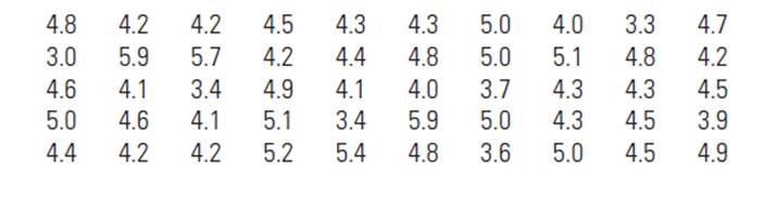
The below is the sample means of n=50 selected samples.

   4.8 4.2 4.2 4.5 4.3 4.354 3.3 4.73 5.9 5.7 4.2 4.4 4.85 5.1 4.8 4.2 4.6 4.1 3.4 4.9 4.14 3.7 4.3 4.3 4.55 4.6 4.1 5.1 3.4 5.95 4.3 4.5 3.9 4.4 4.2 4.2 5.2 5.4 4.8 3.65 4.5 4.9

Calculation:

Let the class intervals as >2.85 and 3.15,>3.15 and 3.45,...>5.85 and 6.15 .

The probability is the frequency divided by the total number of samples.

The below table gives the probability for each class.

  Class Mid value Frequency Probability>2.85 and3.15        3                  1                  0.02>3.15 and3.45        3.3               3                  0.06>3.45 and3.75        3.6               2                  0.04>3.75 and4.05        3.9               3                  0.06>4.05 and4.35        4.2              14                 0.28>4.35 and4.65        4.5               8                  0.16>4.65 and4.95        4.8               7                  0.14>4.95 and5.25        5.1               8                  0.16>5.25 and5.55        5.4               1                  0.02>5.55 and5.85        5.7               1                  0.02>5.85 and6.15        5.7               2                  0.04

Graph:

Below is the histogram of sample means, the vertical axis represents the percentage and the horizontal axis represents the midpoints of the sample mean classes.
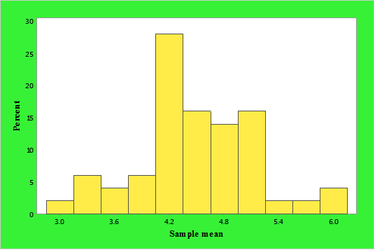
  EBK INTRODUCTION TO PROBABILITY AND STA, Chapter 7.5, Problem 7.17E , additional homework tip  2

Interpretation:

From the above histogram, it can say that the distribution of the sample means is approximately mound-shaped.

Want to see more full solutions like this?

Subscribe now to access step-by-step solutions to millions of textbook problems written by subject matter experts!

Chapter 7 Solutions

EBK INTRODUCTION TO PROBABILITY AND STA

Knowledge Booster
Background pattern image
Statistics
Learn more about
Need a deep-dive on the concept behind this application? Look no further. Learn more about this topic, statistics and related others by exploring similar questions and additional content below.
Recommended textbooks for you
Text book image
Glencoe Algebra 1, Student Edition, 9780079039897...
Algebra
ISBN:9780079039897
Author:Carter
Publisher:McGraw Hill
Statistics 4.1 Point Estimators; Author: Dr. Jack L. Jackson II;https://www.youtube.com/watch?v=2MrI0J8XCEE;License: Standard YouTube License, CC-BY
Statistics 101: Point Estimators; Author: Brandon Foltz;https://www.youtube.com/watch?v=4v41z3HwLaM;License: Standard YouTube License, CC-BY
Central limit theorem; Author: 365 Data Science;https://www.youtube.com/watch?v=b5xQmk9veZ4;License: Standard YouTube License, CC-BY
Point Estimate Definition & Example; Author: Prof. Essa;https://www.youtube.com/watch?v=OTVwtvQmSn0;License: Standard Youtube License
Point Estimation; Author: Vamsidhar Ambatipudi;https://www.youtube.com/watch?v=flqhlM2bZWc;License: Standard Youtube License