ML_assignment_6
.pdf
keyboard_arrow_up
School
Drexel University *
*We aren’t endorsed by this school
Course
613
Subject
Computer Science
Date
Feb 20, 2024
Type
Pages
5
Uploaded by CaptainMantisMaster961
Your preview ends here
Eager to read complete document? Join bartleby learn and gain access to the full version
- Access to all documents
- Unlimited textbook solutions
- 24/7 expert homework help
Recommended textbooks for you
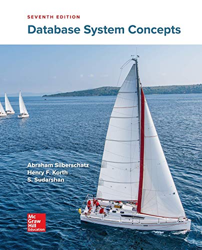
Database System Concepts
Computer Science
ISBN:9780078022159
Author:Abraham Silberschatz Professor, Henry F. Korth, S. Sudarshan
Publisher:McGraw-Hill Education
Starting Out with Python (4th Edition)
Computer Science
ISBN:9780134444321
Author:Tony Gaddis
Publisher:PEARSON

Digital Fundamentals (11th Edition)
Computer Science
ISBN:9780132737968
Author:Thomas L. Floyd
Publisher:PEARSON
C How to Program (8th Edition)
Computer Science
ISBN:9780133976892
Author:Paul J. Deitel, Harvey Deitel
Publisher:PEARSON
Database Systems: Design, Implementation, & Manag...
Computer Science
ISBN:9781337627900
Author:Carlos Coronel, Steven Morris
Publisher:Cengage Learning
Programmable Logic Controllers
Computer Science
ISBN:9780073373843
Author:Frank D. Petruzella
Publisher:McGraw-Hill Education
Recommended textbooks for you
 Database System ConceptsComputer ScienceISBN:9780078022159Author:Abraham Silberschatz Professor, Henry F. Korth, S. SudarshanPublisher:McGraw-Hill Education
 Starting Out with Python (4th Edition)Computer ScienceISBN:9780134444321Author:Tony GaddisPublisher:PEARSON
 Digital Fundamentals (11th Edition)Computer ScienceISBN:9780132737968Author:Thomas L. FloydPublisher:PEARSON
 C How to Program (8th Edition)Computer ScienceISBN:9780133976892Author:Paul J. Deitel, Harvey DeitelPublisher:PEARSON
 Database Systems: Design, Implementation, & Manag...Computer ScienceISBN:9781337627900Author:Carlos Coronel, Steven MorrisPublisher:Cengage Learning
 Programmable Logic ControllersComputer ScienceISBN:9780073373843Author:Frank D. PetruzellaPublisher:McGraw-Hill Education

Database System Concepts
Computer Science
ISBN:9780078022159
Author:Abraham Silberschatz Professor, Henry F. Korth, S. Sudarshan
Publisher:McGraw-Hill Education

Starting Out with Python (4th Edition)
Computer Science
ISBN:9780134444321
Author:Tony Gaddis
Publisher:PEARSON

Digital Fundamentals (11th Edition)
Computer Science
ISBN:9780132737968
Author:Thomas L. Floyd
Publisher:PEARSON

C How to Program (8th Edition)
Computer Science
ISBN:9780133976892
Author:Paul J. Deitel, Harvey Deitel
Publisher:PEARSON

Database Systems: Design, Implementation, & Manag...
Computer Science
ISBN:9781337627900
Author:Carlos Coronel, Steven Morris
Publisher:Cengage Learning

Programmable Logic Controllers
Computer Science
ISBN:9780073373843
Author:Frank D. Petruzella
Publisher:McGraw-Hill Education