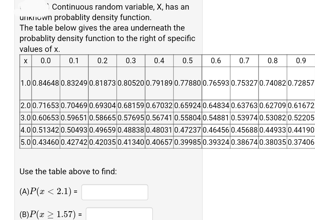
Continuous random variable, X, has an uNKnOwn probablity density function. The table below gives the area underneath the probablity density function to the right of specific values of x. X 0.0 0.1 0.2 0.3 0.4 0.5 0.6 0.7 0.8 0.9 1.00.84648 0.83249 0.81873 0.80520 0.79189 0.778800.76593 0.75327 0.74082 0.72857 2.00.71653 0.70469 0.69304 0.68159 0.67032 0.659240.64834 0.637630.62709 0.61672 3.00.60653 0.59651 0.586650.576950.56741 0.558040.54881 0.53974 0.53082 0.52205 4.00.51342 0.50493 0.49659 0.48838 0.48031 0.47237 0.46456 0.45688 0.44933 0.44190 5.00.43460 0.42742 0.420350.41340 0.40657 0.399850.39324 0.38674 0.38035 0.37406 Use the table above to find: (A)P(x < 2.1) = (B)P(x > 1.57) =

Let x be a continuous random variable that follows a normal distribution with a mean of 200 and a standard deviation of 26. Find the value of x so that the area under the normal curve to the left of x is approximately 0.9924.Round your answer to two decimal places.

Draw the standard normal curve that corresponds to an area between z = 0 and z = 2. Then, use the standard normal table to find the area under the curve between these two z-scores.

Below is a graph of a normal distribution with mean =μ1 and standard deviation =σ4. The shaded region represents the probability of obtaining a value from this distribution that is between 3and 5.   0.1 0.2 0.3 0.4 X 1 3 5     Shade the corresponding region under the standard normal density curve below.   0.1 0.2 0.3 0.4 Z 1 2 3 4 5 6 7 8 9 -1 -2 -3 -4 -5 -6 -7 -8 -9

Solve for D

Find the area under the standard normal curve to the right of z = 2.04 z= 1.09 Genetics: Pea plants contain two genes for seed color, each of which may be Y (for yellow seeds) or G (for green seeds). Plants that contain one of each type of gene are called heterozygous. According to the Mendelian theory of genetics, if two heterozygous plants are crossed, each of their offspring will have probability 0.75 of having yellow seeds and probability 0.25 of having green seeds. One hundred such offspring are produced. Approximate the probability that more than 30 have green seeds.

Determine the area under the standard normal curve that lies to the right of the z-score 0.05 and to the left of the z-score 0.25. z−0.2−0.10.00.10.20.30.40.50.000.42070.46020.50000.53980.57930.61790.65540.69150.010.41680.45620.50400.54380.58320.62170.65910.69500.020.41290.45220.50800.54780.58710.62550.66280.69850.030.40900.44830.51200.55170.59100.62930.66640.70190.040.40520.44430.51600.55570.59480.63310.67000.70540.050.40130.44040.51990.55960.59870.63680.67360.70880.060.39740.43640.52390.56360.60260.64060.67720.71230.070.39360.43250.52790.56750.60640.64430.68080.71570.080.38970.42860.53190.57140.61030.64800.68440.71900.090.38590.42470.53590.57530.61410.65170.68790.7224 Use the value(s) from the table above.