
MATLAB: An Introduction with Applications
6th Edition
ISBN: 9781119256830
Author: Amos Gilat
Publisher: John Wiley & Sons Inc
expand_more
expand_more
format_list_bulleted
Related questions
Question
The
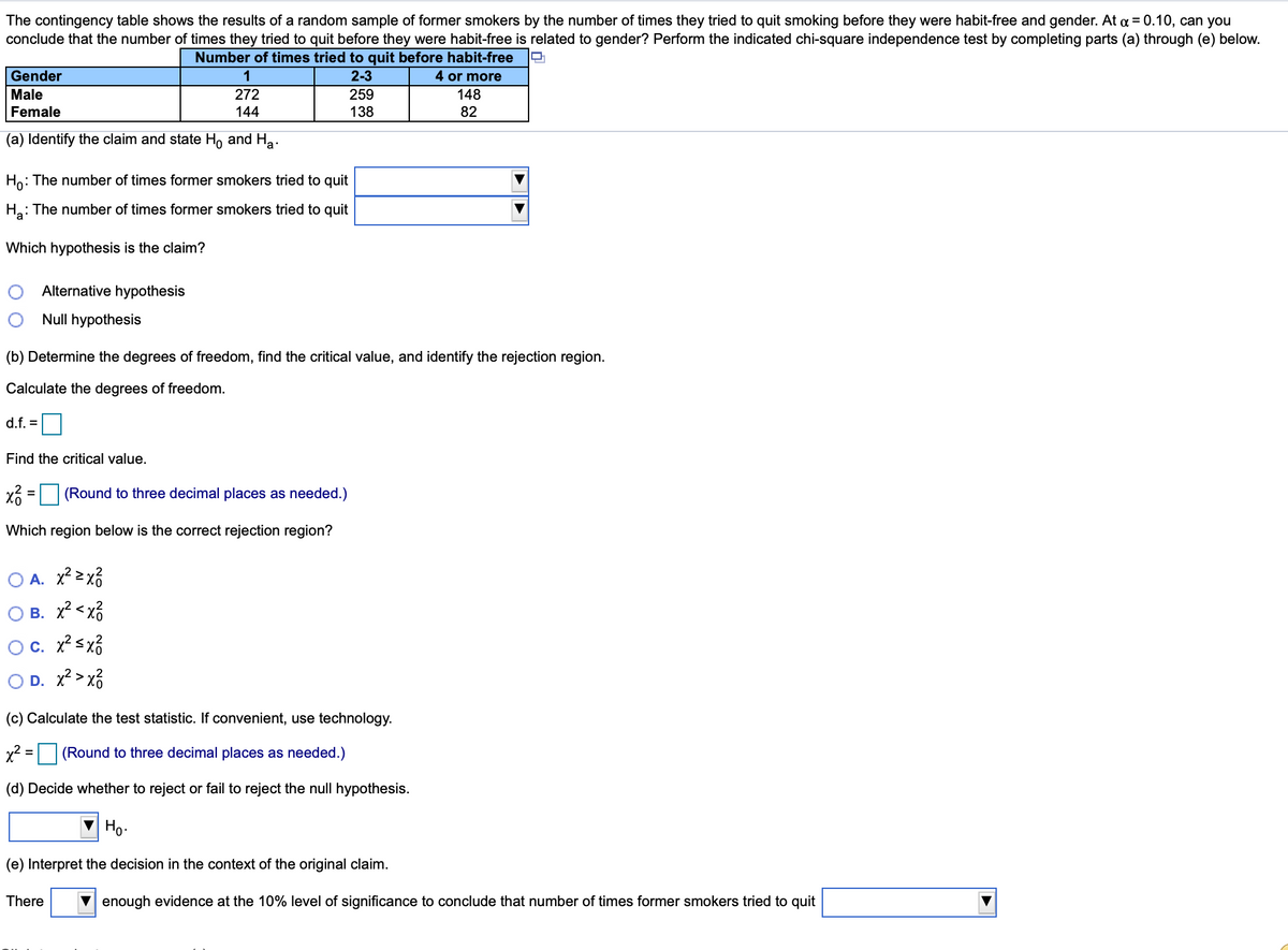

Transcribed Image Text:The contingency table shows the results of a random sample of former smokers by the number of times they tried to quit smoking before they were habit-free and gender. At a = 0.10, can you
conclude that the number of times they tried to quit before they were habit-free is related to gender? Perform the indicated chi-square independence test by completing parts (a) through (e) below.
Number of times tried to quit before habit-free
Gender
1
2-3
4 or more
Male
272
259
148
Female
144
138
82
(a) Identify the claim and state H, and Ha.
Ho: The number of times former smokers tried to quit
H.: The number of times former smokers tried to quit
Which hypothesis is the claim?
Alternative hypothesis
Null hypothesis
(b) Determine the degrees of freedom, find the critical value, and identify the rejection region.
Calculate the degrees of freedom.
d.f. =
Find the critical value.
x =(Round to three decimal places as needed.)
%3D
Which region below is the correct rejection region?
A. x² >x3
B. x? < xổ
c. x? sx3
O D. x? > x3
(c) Calculate the test statistic. If convenient, use technology.
x2 = (Round to three decimal places as needed.)
(d) Decide whether to reject or fail to reject the null hypothesis.
V Ho.
(e) Interpret the decision in the context of the original claim.
There
enough evidence at the 10% level of significance to conclude that number of times former smokers tried to quit
Expert Solution
This question has been solved!
Explore an expertly crafted, step-by-step solution for a thorough understanding of key concepts.

This is a popular solution

Trending nowThis is a popular solution!

Step by stepSolved in 3 steps

Knowledge Booster


Learn more about
Need a deep-dive on the concept behind this application? Look no further. Learn more about this topic, statistics and related others by exploring similar questions and additional content below.Similar questions
- The U.S. Department of Transportation, National Highway Traffic Safety Administration, reported that 77% of all fatally injured automobile drivers were intoxicated. A random sample of 52 records of automobile driver fatalities in a certain county showed that 33 involved an intoxicated driver. Do these data indicate that the population proportion of driver fatalities related to alcohol is less than 77% in Kit Carson County? Use ? = 0.05. (a) level of significance: .05 | H0: p = 0.77; H1: p < 0.77 (b) The standard normal, since np > 5 and nq > 5. What is the value of the sample test statistic? (Round your answer to two decimal places.) Find the P-value of the test statistic. (Round your answer to four decimal places.)arrow_forwardAn automobile dealer conducted a test to determine if the time in minutes needed to complete a minor engine tune-up depends on whether a computerized engine analyzer or an electronic analyzer is used. Because tune-up time varies among compact, intermediate, and full-sized cars, the three types of cars were used as blocks in the experiment. The data obtained follow. Analyzer Computerized Electronic Compact 50 41 Car Intermediate 56 44 Full-sized 62 47 Use a = 0.05 to test for any significant differences. State the null and alternative hypotheses. O Ho: Hcompact * HIntermediate * HFull-sized Ha: "Compact = HIntermediate = 4Full-sized O Ho: HComputerized * HElectronic Ha: HComputerized = HElectronic O Ho: HComputerized = HElectronic Ha: "Computerized * HElectronic O Ho: HComputerized = HElectronic = "Compact = HIntermediate = "Full-sized H.: Not all the population means are equal. O Ho: HCompact = HIntermediate = HFull-sized Hai H compact * HIntermediate * HFull-sized Find the value of…arrow_forwardshow full work for psych statsarrow_forward
- It has been claimed that at UCLA at least 40% of the students live on campus. In a random sample of 250 students, 90 were found to live on campus. Does the evidence support the claim at = .01?arrow_forwardA 2019 study surveyed Norwegian parents about their children's eating habits and taste sensitivities. We are interested in seeing if there is a relationship between sensitivity to sweetness and emotional overeating. The study reports an F* = 2.34 with dfb 3 and dfw = 96. How many levels of 'sensitivity to sweetness' were used in the study? How many subjects participated in the entire study?arrow_forwardTime to Complete the Course Right 45 47 50 49 50 50 48 44 Left | 45 | 43 48 47 50 52 | 44 42 Assume a Normal distribution. What can be concluded at the the a = 0.01 level of significance level of significance? For this study, we should use t-test for the difference between two dependent population means a. The null and alternative hypotheses would be: p1 p2 Ні: p1 p2 b. The test statistic t v v = 1.199 (please show your answer to 3 decimal places.) c. The p-value = [1338 your answer to 4 decimal places.) d. The p-value is > va e. Based on this, we should fail to reject f. Thus, the final conclusion is that ... * (Please show v the null hypothesis. O The results are statistically insignificant at a = 0.01, so there is insufficient evidence to conclude that the population mean time to complete the obstacle course with a patch overarrow_forward
- Calculate the X² statistic, degree of freedom and critical value.arrow_forwardRecent results suggest that children with ADHD tend to watch more TV than children who are not diagnosed with the disorder. To examine this relationship, a researcher obtains a random sample of n = 36 children, 8 to 12 years old, who have been diagnosed with ADHD. Each child is asked to keep a journal recording how much time each day is spent watching TV. The average daily time for the sample is M = 4.9 hours. It is known that the average time for the general population of 8 to 12-year-old children is = 4.1 hours with = 1.8. (Hint: Be sure to use the correct test statistic). Are the data sufficient to conclude that children with ADHD watch significantly more TV than children without the disorder? Use a two-tailed test with = .05. (Be sure to give your conclusion, too) If the researcher had used a sample of n = 9 children and obtained the same sample mean, would the results be sufficient to reject H0? (Be sure to give your conclusion, too) Compute Cohen's d for this study. What is…arrow_forward
arrow_back_ios
arrow_forward_ios
Recommended textbooks for you
- MATLAB: An Introduction with ApplicationsStatisticsISBN:9781119256830Author:Amos GilatPublisher:John Wiley & Sons Inc
 Probability and Statistics for Engineering and th...StatisticsISBN:9781305251809Author:Jay L. DevorePublisher:Cengage Learning
 Statistics for The Behavioral Sciences (MindTap C...StatisticsISBN:9781305504912Author:Frederick J Gravetter, Larry B. WallnauPublisher:Cengage Learning
  Elementary Statistics: Picturing the World (7th E...StatisticsISBN:9780134683416Author:Ron Larson, Betsy FarberPublisher:PEARSON
 The Basic Practice of StatisticsStatisticsISBN:9781319042578Author:David S. Moore, William I. Notz, Michael A. FlignerPublisher:W. H. Freeman
 Introduction to the Practice of StatisticsStatisticsISBN:9781319013387Author:David S. Moore, George P. McCabe, Bruce A. CraigPublisher:W. H. Freeman
MATLAB: An Introduction with Applications
Statistics
ISBN:9781119256830
Author:Amos Gilat
Publisher:John Wiley & Sons Inc
Probability and Statistics for Engineering and th...
Statistics
ISBN:9781305251809
Author:Jay L. Devore
Publisher:Cengage Learning
Statistics for The Behavioral Sciences (MindTap C...
Statistics
ISBN:9781305504912
Author:Frederick J Gravetter, Larry B. Wallnau
Publisher:Cengage Learning
Elementary Statistics: Picturing the World (7th E...
Statistics
ISBN:9780134683416
Author:Ron Larson, Betsy Farber
Publisher:PEARSON
The Basic Practice of Statistics
Statistics
ISBN:9781319042578
Author:David S. Moore, William I. Notz, Michael A. Fligner
Publisher:W. H. Freeman
Introduction to the Practice of Statistics
Statistics
ISBN:9781319013387
Author:David S. Moore, George P. McCabe, Bruce A. Craig
Publisher:W. H. Freeman