Concept explainers
Videos
For Exercises 1 through 7, do a complete
a. Draw the
b. Compute the value of the
c. Test the significance of the correlation coefficient at α = 0.01, using Table I.
d. Determine the regression line equation if r is significant.
e. Plot the regression line on the scatter plot, if appropriate.
f. Predict y′ for a specific value of x, if appropriate.
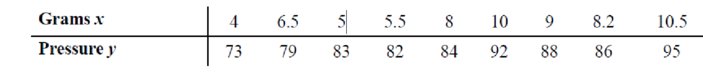
6. Protein and Diastolic Blood Pressure A study was conducted with vegetarians to see whether the number of grams of protein each ate per day was related to diastolic blood pressure. The data are given here. If there is a significant relationship, predict the diastolic pressure of a vegetarian who consumes 8 grams of protein per day. (This information will be used for Exercises 10 and 12.)
a.
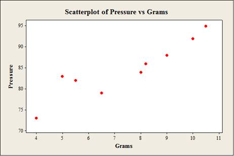
To construct: The scatterplot for the variables the number of grams of protein and the diastolic blood pressure.
Answer to Problem 10.1.6RE
Output using the MINITAB software is given below:
Explanation of Solution
Given info:
The data shows the number of grams of protein (x) and the diastolic blood pressure (y) values.
Calculation:
Step by step procedure to obtain scatterplot using the MINITAB software:
- Choose Graph > Scatterplot.
- Choose Simple and then click OK.
- Under Y variables, enter a column of Pressure.
- Under X variables, enter a column of Grams.
- Click OK.
b.
To compute: The value of the correlation coefficient.
Answer to Problem 10.1.6RE
The value of the correlation coefficient is 0.916.
Explanation of Solution
Calculation:
Correlation coefficient r:
Software Procedure:
Step-by-step procedure to obtain the ‘correlation coefficient’ using the MINITAB software:
- Select Stat > Basic Statistics > Correlation.
- In Variables, select x and y from the box on the left.
- Click OK.
Output using the MINITAB software is given below:
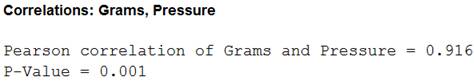
From the MINITAB output, the value of the correlation is 0.916.
c.
To test: The significance of the correlation coefficient at
Answer to Problem 10.1.6RE
The conclusion is that, there is a linear relation between the number of grams of protein and the diastolic blood pressure.
Explanation of Solution
Given info:
The level of significance is
Calculation:
The hypotheses are given below:
Null hypothesis:
That is, there is no linear relation between the number of grams of protein and the diastolic blood pressure.
Alternative hypothesis:
That is, there is a linear relation between the number of grams of protein and the diastolic blood pressure.
The sample size is 9.
The formula to find the degrees of the freedom is
That is,
From the “TABLE –I: Critical Values for the PPMC”, the critical value for 7 degrees of freedom and
Rejection Rule:
If the absolute value of r is greater than the critical value then reject the null hypothesis.
Conclusion:
From part (b), the value of r is 0.916 that is the absolute value of r is 0.916.
Here, the absolute value of r is greater than the critical value
That is,
By the rejection rule, reject the null hypothesis.
There is a sufficient evidence to support the claim that “there is a linear relation between the number of grams of protein and the diastolic blood pressure.
d.
To find: The regression equation for the given data.
Answer to Problem 10.1.6RE
The regression equation for the given data is
Explanation of Solution
Calculation:
Regression:
Software procedure:
Step by step procedure to obtain the regression equation using the MINITAB software:
- Choose Stat > Regression > Regression.
- In Responses, enter the column of Pressure.
- In Predictors, enter the column of Grams.
- Click OK.
Output using the MINITAB software is given below:
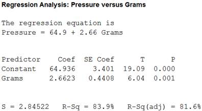
Thus, regression equation for the given data is
e.
To construct: The scatterplot for the variables the speed and time with regression line.
Answer to Problem 10.1.6RE
Output using the MINITAB software is given below:

Explanation of Solution
Calculation:
Step by step procedure to obtain scatterplot using the MINITAB software:
- Choose Graph > Scatterplot.
- Choose with line and then click OK.
- Under Y variables, enter a column of Pressure.
- Under X variables, enter a column of Grams.
- Click OK.
f.
To obtain: The predicted value of the diastolic pressure of a vegetarian who consumes 8 grams of protein per day.
Answer to Problem 10.1.6RE
The predicted value of the diastolic pressure of a vegetarian is 86.232.
Explanation of Solution
Calculation:
Thus, regression equation for the given data is
Substitute x as 8 in the regression equation
Thus, the predicted value of the diastolic pressure of a vegetarian is 86.232.
Want to see more full solutions like this?
Chapter 10 Solutions
Loose Leaf Elementary Statistics: A Step By Step Approach With Connect Math Hosted By Aleks Access Card


- For the following exercises, consider the data in Table 5, which shows the percent of unemployed ina city of people 25 years or older who are college graduates is given below, by year. 40. Based on the set of data given in Table 6, calculate the regression line using a calculator or other technology tool, and determine the correlation coefficient to three decimal places.arrow_forwardFor the following exercises, consider the data in Table 5, which shows the percent of unemployed in a city ofpeople25 years or older who are college graduates is given below, by year. 41. Based on the set of data given in Table 7, calculatethe regression line using a calculator or othertechnology tool, and determine the correlationcoefficient to three decimal places.arrow_forwardThe following fictitious table shows kryptonite price, in dollar per gram, t years after 2006. t= Years since 2006 0 1 2 3 4 5 6 7 8 9 10 K= Price 56 51 50 55 58 52 45 43 44 48 51 Make a quartic model of these data. Round the regression parameters to two decimal places.arrow_forward
- For the following exercises, use Table 4 which shows the percent of unemployed persons 25 years or older who are college graduates in a particular city, by year. Based on the set of data given in Table 5, calculate the regression line using a calculator or other technology tool, and determine the correlation coefficient. Round to three decimal places of accuracyarrow_forwardRun a regression analysis on the following data set, where yy is the final grade in a math class and xx is the average number of hours the student spent working on math each week. hours/weekx Gradey 5 59 6 54.4 6 56.4 8 59.2 11 68.4 12 78.8 13 75.2 14 89.6 14 89.6 16 87.4 State the regression equation y=m⋅x+by=m⋅x+b, with constants accurate to two decimal places. What is the predicted value for the final grade when a student spends an average of 15 hours each week on math?Grade = Round to 1 decimal place.arrow_forwardConsider the following data set, where yy is the final grade in a math class and xx is the average number of hours the student spent working on math each week. hours/weekx Gradey 5 58 8 63.2 8 73.2 9 68.6 9 70.6 11 68.4 13 81.2 14 86.6 17 100 20 100 The regression equation is y=3.04⋅x+42.33y=3.04⋅x+42.33.Explain what the value of the slope means in this situation, where yy is the final grade in a math class and xx is the average number of hours the student spent working on math each week.Explain what the value of the y-intercept means in this situation.What is the predicted value for the final grade when a student spends an average of 15 hours each week on math?Grade = Round to 1 decimal place.arrow_forward
- For the following data: a. Find the regression equation for predicting Y from X. b. Calculate the Pearson correlation for these data. Use r2 and SSY to compute SSresidual and the standard error of estimate for the equation. X Y 3 3 6 9 5 8 4 3 7 10 5 9 c. Slope equation: Y= _______ X+ _________ d. r= e. r2= f. SSY= g. SSRes= h. SEEst=arrow_forwardConsider the following data: A. Find the equation of the regression line. B. Draw the graph of the regression equation on the scatter plot. x 1 2 3 4 5 6 7 y 15 10 20 5 25 20 35arrow_forwardThere is a relation between the following variables as y = 1 / (a * x ^ b) (x ^ b means x over b) a) Calculate the correlation coefficient and interpret the degree of the relationship? b) Estimate the y-value for x = 4.3 and the x-value for y = 0.90 by obtaining the regression equationarrow_forward
- Consider the following regression equation representing the linear relationship between the Canada Child Benefit provided for a married couple with 3 children under the age of 6, based on their annual family net income: ŷ =121.09−0.57246xR2=0.894 where y = annual Canada Child Benefit paid (in $100s) x = net annual family income (in $1000s) Source: Canada Revenue Agency a. As the net annual family income increases, does the Canada Child Benefit paid increase or decrease? Based on this, is the correlation between the two variables positive or negative?The Canada Child Benefit paid .The correlation between the two variables is .b. Calculate the correlation coefficient and determine if the relationship between the two variables is strong, moderate or weak.r= , the relationship is . Round to 3 decimal places c. Interpret the value of the slope as it relates to this relationship. For every $1 increase in annual family net income, there is a $0.57246 decrease in…arrow_forwardConsider the following regression equation representing the linear relationship between the Canada Child Benefit provided for a married couple with 3 children under the age of 6, based on their annual family net income: ŷ =121.09−0.57246xR2=0.894 where y= annual Canada Child Benefit paid (in $100s) x = net annual family income (in $1000s) Source: Canada Revenue Agency a. As the net annual family income increases, does the Canada Child Benefit paid increase or decrease? Based on this, is the correlation between the two variables positive or negative?The Canada Child Benefit paid ? .The correlation between the two variables is ? .b. Calculate the correlation coefficient and determine if the relationship between the two variables is strong, moderate or weak.r= , the relationship is ? . Round to 3 decimal places c. Interpret the value of the slope as it relates to this relationship. For every $1 increase in annual family net income, there is a $0.57246 decrease in…arrow_forwardThe following table shows the annual expenditures, in dollars, per customer unit for residential landline phone services and cellular phone services in the United States in the given year.† Year Landline Cell 2004 592 378 2006 542 524 2008 467 643 2010 401 760 Calculate the regression line for each type of service. (Let t be the time in years since 2004, L be the operating revenue of landline phone services and C be the expenditure of cellular services. Round your regression parameters to two decimal places.) L(t) = C(t) = Determine the expenditure level at which the two lines cross. Round your answer for the expenditure level to one decimal place. million dollarsarrow_forward
 Algebra and Trigonometry (MindTap Course List)AlgebraISBN:9781305071742Author:James Stewart, Lothar Redlin, Saleem WatsonPublisher:Cengage Learning
 Functions and Change: A Modeling Approach to Coll...AlgebraISBN:9781337111348Author:Bruce Crauder, Benny Evans, Alan NoellPublisher:Cengage Learning