Chapter 10, Problem 10.34P

To determine

(a)

The values of gain $K_P\text{and}{K}_I$ of the PI controller of first-order plant for the following collection of roots:

Case 1. For $s=-2,-20$ (Root separation factor is 10).

Case 2. For $s=-2,-10$ (Root separation factor is 5).

Case 3. For $s=-2,-4$ (Root separation factor is 2).

Answer to Problem 10.34P

The values of gains for the PI controller are as follows:

Case 1. For $s=-2,-20$, $K_I=200$ and $K_P=106$.

Case 2. For $s=-2,-10$, $K_I=100$ and $K_P=56$.

Case 3. For $s=-2,-4$, $K_I=40$ and $K_P=26$.

Explanation of Solution

Given:

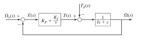
The proportional integral controller of first order plant is as shown below:

Where, the parameter values are as given:

$I=5,c=4$

Also, the performance specifications require the time constant of the system to be $\tau =0.5$.

Concept Used:

1. The transfer functions for the block diagram are as shown below:

$\begin{array}{l}\frac{\Omega \left(s\right)}{{\Omega }_r\left(s\right)}=\frac{s{K}_P+K_I}{I{s}^2+s\left(c+K_P\right)+K_I}\\ \frac{\Omega \left(s\right)}{T_d\left(s\right)}=\frac{-s}{I{s}^2+s\left(c+K_P\right)+K_I}\end{array}$

2. For a second order system having a characteristic equation of the form $s^2+2\zeta {\omega }_{n}s+{\omega }_n{}^2=0$, the characteristic roots are of the form $s=-\zeta {\omega }_{n}s\pm {\omega }_n\sqrt{1-{\zeta }^2}\forall \zeta \le 1$ .

Also, the corresponding time constant for the system would be $\tau =\frac{1}{\zeta {\omega }_n}$.

3. For a second order system, if the root separation factor is K then, we have following conclusions for the roots and their corresponding time constant, that is
For roots $s_1\text{and}{s}_2$ ,

$\frac{s_1}{s_2}=K$

The corresponding time constants of the system would be:

$\frac{{\tau }_1}{{\tau }_2}=\frac{\frac{1}{\mathrm{Re}\left(s_1\right)}}{\frac{1}{\mathrm{Re}\left(s_2\right)}}=\frac{\mathrm{Re}\left(s_2\right)}{\mathrm{Re}\left(s_1\right)}=\frac{1}{K}$

Calculation:

From the block diagram as shown, the transfer functions are as:

$\begin{array}{l}\frac{\Omega \left(s\right)}{{\Omega }_r\left(s\right)}=\frac{s{K}_P+K_I}{I{s}^2+s\left(c+K_P\right)+K_I}\\ \frac{\Omega \left(s\right)}{T_d\left(s\right)}=\frac{-s}{I{s}^2+s\left(c+K_P\right)+K_I}\end{array}$

Therefore, the characteristic equation for the system is:

$I{s}^2+s\left(c+K_P\right)+K_I=0$

On putting the values of parameters in this expression of characteristic equation:

$\begin{array}{l}I{s}^2+s\left(c+K_P\right)+K_I=0\\ \Rightarrow 5s^2+s\left(4+K_P\right)+K_I=0\because I=5,c=4\\ \Rightarrow s^2+s\frac{\left(4+K_P\right)}{5}+\frac{K_I}{5}=0\end{array}$

Case 1. When the root separation factor is 10.

The given set of roots for this root separation are:

$s=-2,s=-20$

Thus, the corresponding characteristic equation for the system will be:

$\begin{array}{l}s=-2,s=-20\\ \Rightarrow \left(s+2\right)\left(s+20\right)=0\\ \Rightarrow s^2+22s+40=0\end{array}$

On comparing this equation with $s^2+s\frac{\left(4+K_P\right)}{5}+\frac{K_I}{5}=0$, we get

$\begin{array}{l}\frac{K_I}{5}=40\\ \Rightarrow K_I=200\end{array}$

And

$\begin{array}{l}\frac{\left(4+K_P\right)}{5}=22\\ \Rightarrow 4+K_P=110\\ \Rightarrow K_P=106\end{array}$

Case 2. When the root separation factor is 5.

The given set of roots for this root separation are:

$s=-2,s=-10$

Thus, the corresponding characteristic equation for the system will be:

$\begin{array}{l}s=-2,s=-10\\ \Rightarrow \left(s+2\right)\left(s+10\right)=0\\ \Rightarrow s^2+12s+20=0\end{array}$

On comparing this equation with $s^2+s\frac{\left(4+K_P\right)}{5}+\frac{K_I}{5}=0$, we get

$\begin{array}{l}\frac{K_I}{5}=20\\ \Rightarrow K_I=100\end{array}$

And

$\begin{array}{l}\frac{\left(4+K_P\right)}{5}=12\\ \Rightarrow 4+K_P=60\\ \Rightarrow K_P=56\end{array}$

Case 3. When the root separation factor is 2.

The given set of roots for this root separation are:

$s=-2,s=-4$

Thus, the corresponding characteristic equation for the system will be:

$\begin{array}{l}s=-2,s=-4\\ \Rightarrow \left(s+2\right)\left(s+4\right)=0\\ \Rightarrow s^2+6s+8=0\end{array}$

On comparing this equation with $s^2+s\frac{\left(4+K_P\right)}{5}+\frac{K_I}{5}=0$, we get

$\begin{array}{l}\frac{K_I}{5}=8\\ \Rightarrow K_I=40\end{array}$

And

$\begin{array}{l}\frac{\left(4+K_P\right)}{5}=6\\ \Rightarrow 4+K_P=30\end{array}$

$\Rightarrow K_P=26$.

Conclusion:

The values of gains for the PI controller are as follows:

Case 1. For $s=-2,-20$, $K_I=200$ and $K_P=106$.

Case 2. For $s=-2,-10$, $K_I=100$ and $K_P=56$.

Case 3. For $s=-2,-4$, $K_I=40$ and $K_P=26$.

To determine

(b)

To plot:

The response $\omega \left(t\right)$ for the unit-step command response ${\omega }_r\left(t\right)$ for all the cases in sub-part (a)

Also, discuss the impact of root separation factor on the responses obtained in all these cases through the perspective of rise time, the overshoot and the maximum required torque.

Answer to Problem 10.34P

The response, $\omega \left(t\right)$ ,for the unit-step command response, ${\omega }_r\left(t\right)$, for all the cases in sub-part (a) is shown in Figure 1.

The impact of root separation factor are as follows:

Case 1. For $s=-2,-20$ (Root separation factor is 10), $t_r\approx 0.15\text{seconds}$, $T_m\approx 106\text{N}\cdot \text{m}$ and $M_P\approx 1.034\text{units}$.

Case 2. For $s=-2,-10$ (Root separation factor is 5), $t_r\approx 0.25\text{seconds}$, $T_m\approx 56\text{N}\cdot \text{m}$ and $M_P\approx 1.048\text{units}$.

Case 3. For $s=-2,-4$ (Root separation factor is 2), $t_r\approx 0.49\text{seconds}$, $T_m\approx 26\text{N}\cdot \text{m}$ and $M_P\approx 1.055\text{units}$.

Thus, we see that with decrease in the root separation factor, the rise time as well as the overshoot increases. While for the required torque, the value of maximum torque decreased with increased root separation factor.

Explanation of Solution

Given:

The proportional integral controller of first order plant is as shown below:

Where, the parameter values are as given:

$I=5,c=4$

Also, the performance specifications require the time constant of the system to be $\tau =0.5$.

The values of gains for the PI controller are as follows:

Case 1. For $s=-2,-20$, $K_I=200$ and $K_P=106$.

Case 2. For $s=-2,-10$, $K_I=100$ and $K_P=56$.

Case 3. For $s=-2,-4$, $K_I=40$ and $K_P=26$.

Concept Used:

1. The transfer functions for the block diagram are as shown below:

$\begin{array}{l}\frac{\Omega \left(s\right)}{{\Omega }_r\left(s\right)}=\frac{s{K}_P+K_I}{I{s}^2+s\left(c+K_P\right)+K_I}\\ \frac{\Omega \left(s\right)}{T_d\left(s\right)}=\frac{-s}{I{s}^2+s\left(c+K_P\right)+K_I}\end{array}$

Calculation:

From the block diagram as shown, the transfer functions are as:

$\begin{array}{l}\frac{\Omega \left(s\right)}{{\Omega }_r\left(s\right)}=\frac{s{K}_P+K_I}{I{s}^2+s\left(c+K_P\right)+K_I}\\ \frac{\Omega \left(s\right)}{T_d\left(s\right)}=\frac{-s}{I{s}^2+s\left(c+K_P\right)+K_I}\end{array}$

Therefore, the response $\Omega \left(s\right)$ for the system is:

$\Omega \left(s\right)=\frac{s{K}_P+K_I}{I{s}^2+s\left(c+K_P\right)+K_I}{\Omega }_r\left(s\right)-\frac{s}{I{s}^2+s\left(c+K_P\right)+K_I}{T}_d\left(s\right)$

On putting the values of parameters in this expression of characteristic equation:

$\begin{array}{l}\Omega \left(s\right)=\frac{s{K}_P+K_I}{I{s}^2+s\left(c+K_P\right)+K_I}{\Omega }_r\left(s\right)-\frac{s}{I{s}^2+s\left(c+K_P\right)+K_I}{T}_d\left(s\right)\\ \Rightarrow \Omega \left(s\right)=\frac{s{K}_P+K_I}{5s^2+s\left(4+K_P\right)+K_I}{\Omega }_r\left(s\right)-\frac{s}{5s^2+s\left(4+K_P\right)+K_I}{T}_d\left(s\right)\because I=5,c=4\end{array}$

And from the block diagram shown in figure, we have

$\begin{array}{l}T\left(s\right)=\left(K_P+\frac{K_I}{s}\right)E\left(s\right)\\ \Rightarrow T\left(s\right)=\left(K_P+\frac{K_I}{s}\right)\left({\Omega }_r\left(s\right)-\Omega \left(s\right)\right)\because E\left(s\right)={\Omega }_r\left(s\right)-\Omega \left(s\right)\\ \Rightarrow T\left(s\right)=\left(K_P+\frac{K_I}{s}\right)\left(\left(1-\frac{s{K}_P+K_I}{I{s}^2+s\left(c+K_P\right)+K_I}\right){\Omega }_r\left(s\right)+\frac{s}{I{s}^2+s\left(c+K_P\right)+K_I}{T}_d\left(s\right)\right)\\ \because \Omega \left(s\right)=\frac{s{K}_P+K_I}{I{s}^2+s\left(c+K_P\right)+K_I}{\Omega }_r\left(s\right)-\frac{s}{I{s}^2+s\left(c+K_P\right)+K_I}{T}_d\left(s\right)\end{array}$

On keeping the values of the parameters such that $I=5,c=4$

$\begin{array}{l}T\left(s\right)=\left(K_P+\frac{K_I}{s}\right)\left(\left(1-\frac{s{K}_P+K_I}{I{s}^2+s\left(c+K_P\right)+K_I}\right){\Omega }_r\left(s\right)+\frac{s}{I{s}^2+s\left(c+K_P\right)+K_I}{T}_d\left(s\right)\right)\\ \Rightarrow T\left(s\right)=\left(K_P+\frac{K_I}{s}\right)\left(\left(\frac{s\left(Is+c\right)}{I{s}^2+s\left(c+K_P\right)+K_I}\right){\Omega }_r\left(s\right)+\frac{s}{I{s}^2+s\left(c+K_P\right)+K_I}{T}_d\left(s\right)\right)\end{array}$

$\Rightarrow T\left(s\right)=\left(K_P+\frac{K_I}{s}\right)\left(\left(\frac{s\left(5s+4\right)}{5s^2+s\left(4+K_P\right)+K_I}\right){\Omega }_r\left(s\right)+\frac{s}{5s^2+s\left(4+K_P\right)+K_I}{T}_d\left(s\right)\right)$

Case 1. For $s=-2,-20$, $K_I=200$ and $K_P=106$:

Since, $\Omega \left(s\right)=\frac{s{K}_P+K_I}{5s^2+s\left(4+K_P\right)+K_I}{\Omega }_r\left(s\right)-\frac{s}{5s^2+s\left(4+K_P\right)+K_I}{T}_d\left(s\right)$

$\begin{array}{l}\Rightarrow \Omega \left(s\right)=\frac{106s+200}{5s^2+s\left(4+106\right)+200}{\Omega }_r\left(s\right)-\frac{s}{5s^2+s\left(4+106\right)+200}{T}_d\left(s\right)\\ \because K_P=106,K_I=200\\ \Rightarrow \Omega \left(s\right)=\frac{106s+200}{5s^2+110s+200}{\Omega }_r\left(s\right)-\frac{s}{5s^2+110s+200}{T}_d\left(s\right)\end{array}$

Therefore, for unit-step command response ${\Omega }_r\left(s\right)$ and zero disturbance torque $T_d\left(s\right)$, we have

$\begin{array}{l}\Omega \left(s\right)=\frac{106s+200}{5s^2+110s+200}{\Omega }_r\left(s\right)-\frac{s}{5s^2+110s+200}{T}_d\left(s\right)\\ \Rightarrow \Omega \left(s\right)=\frac{106s+200}{5s^2+110s+200}\cdot \frac{1}{s}-\frac{s}{5s^2+110s+200}\cdot 0\\ \Rightarrow \Omega \left(s\right)=\frac{106s+200}{5s^2+110s+200}\cdot \frac{1}{s}\end{array}$

On simplifying this response of $\Omega \left(s\right)$ using partial fraction expansion, we get

$\begin{array}{l}\Omega \left(s\right)=\frac{106s+200}{5s^2+110s+200}\cdot \frac{1}{s}\\ \Rightarrow \Omega \left(s\right)=\frac{1}{s}+\frac{1}{15\left(s+2\right)}-\frac{16}{15\left(s+20\right)}\end{array}$

On taking inverse Laplace transform of this, we have

$\begin{array}{l}\Omega \left(s\right)=\frac{1}{s}+\frac{1}{15\left(s+2\right)}-\frac{16}{15\left(s+20\right)}\\ \Rightarrow \omega \left(t\right)=1+\frac{1}{15}{e}^{-2t}-\frac{16}{15}{e}^{-20t}\end{array}$

Also, on keeping the gain values in the expression for torque:

$\begin{array}{l}T\left(s\right)=\left(K_P+\frac{K_I}{s}\right)\left(\left(\frac{s\left(5s+4\right)}{5s^2+s\left(4+K_P\right)+K_I}\right){\Omega }_r\left(s\right)+\frac{s}{5s^2+s\left(4+K_P\right)+K_I}{T}_d\left(s\right)\right)\\ \Rightarrow T\left(s\right)=\left(106+\frac{200}{s}\right)\left(\left(\frac{s\left(5s+4\right)}{5s^2+s\left(4+106\right)+200}\right){\Omega }_r\left(s\right)+\frac{s}{5s^2+s\left(4+106\right)+200}{T}_d\left(s\right)\right)\\ \Rightarrow T\left(s\right)=\left(\left(\frac{\left(106s+200\right)\left(5s+4\right)}{5s^2+110s+200}\right){\Omega }_r\left(s\right)+\frac{\left(106s+200\right)}{5s^2+110s+200}{T}_d\left(s\right)\right)\end{array}$

Therefore, for unit-step command response ${\Omega }_r\left(s\right)$ and zero disturbance torque $T_d\left(s\right)$, we have

$\begin{array}{l}T\left(s\right)=\left(\left(\frac{\left(106s+200\right)\left(5s+4\right)}{5s^2+110s+200}\right){\Omega }_r\left(s\right)+\frac{\left(106s+200\right)}{5s^2+110s+200}{T}_d\left(s\right)\right)\\ \Rightarrow T\left(s\right)=\left(\left(\frac{\left(106s+200\right)\left(5s+4\right)}{5s^2+110s+200}\right)\cdot \frac{1}{s}+\frac{\left(106s+200\right)}{5s^2+110s+200}\cdot 0\right)\\ \Rightarrow T\left(s\right)=\left(\frac{\left(106s+200\right)\left(5s+4\right)}{5s^2+110s+200}\right)\cdot \frac{1}{s}\end{array}$

On simplifying the expression for this torque using partial fraction expansion, we get:

$\begin{array}{l}T\left(s\right)=\left(\frac{\left(106s+200\right)\left(5s+4\right)}{5s^2+110s+200}\right)\cdot \frac{1}{s}\\ \Rightarrow T\left(s\right)=\frac{4}{s}-\frac{2}{5\left(s+2\right)}+\frac{512}{5\left(s+20\right)}\end{array}$

On taking inverse Laplace transform, we have

$\begin{array}{l}T\left(s\right)=\frac{4}{s}-\frac{2}{5\left(s+2\right)}+\frac{512}{5\left(s+20\right)}\\ \Rightarrow T\left(t\right)=4-\frac{2}{5}{e}^{-2t}+\frac{512}{5}{e}^{-20t}\end{array}$

Case 2. For $s=-2,-10$, $K_I=100$ and $K_P=56$:

Since, $\Omega \left(s\right)=\frac{s{K}_P+K_I}{5s^2+s\left(4+K_P\right)+K_I}{\Omega }_r\left(s\right)-\frac{s}{5s^2+s\left(4+K_P\right)+K_I}{T}_d\left(s\right)$

$\Rightarrow \Omega \left(s\right)=\frac{56s+100}{5s^2+s\left(4+56\right)+100}{\Omega }_r\left(s\right)-\frac{s}{5s^2+s\left(4+56\right)+100}{T}_d\left(s\right)$

$\begin{array}{l}\because K_P=56,K_I=100\\ \Rightarrow \Omega \left(s\right)=\frac{56s+100}{5s^2+60s+100}{\Omega }_r\left(s\right)-\frac{s}{5s^2+60s+100}{T}_d\left(s\right)\end{array}$

Therefore, for unit-step command response ${\Omega }_r\left(s\right)$ and zero disturbance torque $T_d\left(s\right)$, we have

$\begin{array}{l}\Omega \left(s\right)=\frac{56s+100}{5s^2+60s+100}{\Omega }_r\left(s\right)-\frac{s}{5s^2+60s+100}{T}_d\left(s\right)\\ \Rightarrow \Omega \left(s\right)=\frac{56s+100}{5s^2+60s+100}\cdot \frac{1}{s}-\frac{s}{5s^2+60s+100}\cdot 0\\ \Rightarrow \Omega \left(s\right)=\frac{56s+100}{5s^2+60s+100}\cdot \frac{1}{s}\end{array}$

On simplifying this response of $\Omega \left(s\right)$ using partial fraction expansion, we get

$\begin{array}{l}\Omega \left(s\right)=\frac{56s+100}{5s^2+60s+100}\cdot \frac{1}{s}\\ \Rightarrow \Omega \left(s\right)=\frac{1}{s}+\frac{3}{20\left(s+2\right)}-\frac{23}{20\left(s+10\right)}\end{array}$

On taking inverse Laplace transform of this, we have

$\begin{array}{l}\Omega \left(s\right)=\frac{1}{s}+\frac{3}{20\left(s+2\right)}-\frac{23}{20\left(s+10\right)}\\ \Rightarrow \omega \left(t\right)=1+\frac{3}{20}{e}^{-2t}-\frac{23}{20}{e}^{-10t}\end{array}$

Also, on keeping the gain values in the expression for torque:

$\begin{array}{l}T\left(s\right)=\left(K_P+\frac{K_I}{s}\right)\left(\left(\frac{s\left(5s+4\right)}{5s^2+s\left(4+K_P\right)+K_I}\right){\Omega }_r\left(s\right)+\frac{s}{5s^2+s\left(4+K_P\right)+K_I}{T}_d\left(s\right)\right)\\ \Rightarrow T\left(s\right)=\left(56+\frac{100}{s}\right)\left(\left(\frac{s\left(5s+4\right)}{5s^2+s\left(4+56\right)+100}\right){\Omega }_r\left(s\right)+\frac{s}{5s^2+s\left(4+56\right)+100}{T}_d\left(s\right)\right)\\ \Rightarrow T\left(s\right)=\left(\left(\frac{\left(56s+100\right)\left(5s+4\right)}{5s^2+60s+100}\right){\Omega }_r\left(s\right)+\frac{\left(56s+100\right)}{5s^2+60s+100}{T}_d\left(s\right)\right)\end{array}$

Therefore, for unit-step command response ${\Omega }_r\left(s\right)$ and zero disturbance torque $T_d\left(s\right)$, we have

$\begin{array}{l}T\left(s\right)=\left(\left(\frac{\left(56s+100\right)\left(5s+4\right)}{5s^2+60s+100}\right){\Omega }_r\left(s\right)+\frac{\left(56s+100\right)}{5s^2+60s+100}{T}_d\left(s\right)\right)\\ \Rightarrow T\left(s\right)=\left(\left(\frac{\left(56s+100\right)\left(5s+4\right)}{5s^2+60s+100}\right)\cdot \frac{1}{s}+\frac{\left(56s+100\right)}{5s^2+60s+100}\cdot 0\right)\\ \Rightarrow T\left(s\right)=\left(\frac{\left(56s+100\right)\left(5s+4\right)}{5s^2+60s+100}\right)\cdot \frac{1}{s}\end{array}$

On simplifying the expression for this torque using partial fraction expansion, we get:

$\begin{array}{l}T\left(s\right)=\left(\frac{\left(56s+100\right)\left(5s+4\right)}{5s^2+60s+100}\right)\cdot \frac{1}{s}\\ \Rightarrow T\left(s\right)=\frac{4}{s}-\frac{9}{10\left(s+2\right)}+\frac{529}{10\left(s+10\right)}\end{array}$

On taking inverse Laplace transform, we have

$\begin{array}{l}T\left(s\right)=\frac{4}{s}-\frac{9}{10\left(s+2\right)}+\frac{529}{10\left(s+10\right)}\\ \Rightarrow T\left(t\right)=4-\frac{9}{10}{e}^{-2t}+\frac{529}{10}{e}^{-10t}\end{array}$

Case 3. For $s=-2,-4$, $K_I=40$ and $K_P=26$:

Since, $\Omega \left(s\right)=\frac{s{K}_P+K_I}{5s^2+s\left(4+K_P\right)+K_I}{\Omega }_r\left(s\right)-\frac{s}{5s^2+s\left(4+K_P\right)+K_I}{T}_d\left(s\right)$

$\begin{array}{l}\Rightarrow \Omega \left(s\right)=\frac{26s+40}{5s^2+s\left(4+26\right)+40}{\Omega }_r\left(s\right)-\frac{s}{5s^2+s\left(4+26\right)+40}{T}_d\left(s\right)\\ \because K_P=26,K_I=40\\ \Rightarrow \Omega \left(s\right)=\frac{26s+40}{5s^2+30s+40}{\Omega }_r\left(s\right)-\frac{s}{5s^2+30s+40}{T}_d\left(s\right)\end{array}$

Therefore, for unit-step command response ${\Omega }_r\left(s\right)$ and zero disturbance torque $T_d\left(s\right)$, we have

$\begin{array}{l}\Omega \left(s\right)=\frac{26s+40}{5s^2+30s+40}{\Omega }_r\left(s\right)-\frac{s}{5s^2+30s+40}{T}_d\left(s\right)\\ \Rightarrow \Omega \left(s\right)=\frac{26s+40}{5s^2+30s+40}\cdot \frac{1}{s}-\frac{s}{5s^2+30s+40}\cdot 0\end{array}$

$\Rightarrow \Omega \left(s\right)=\frac{26s+40}{5s^2+30s+40}\cdot \frac{1}{s}$

On simplifying this response of $\Omega \left(s\right)$ using partial fraction expansion, we get

$\begin{array}{l}\Omega \left(s\right)=\frac{26s+40}{5s^2+30s+40}\cdot \frac{1}{s}\\ \Rightarrow \Omega \left(s\right)=\frac{1}{s}+\frac{3}{5\left(s+2\right)}-\frac{8}{5\left(s+4\right)}\end{array}$

On taking inverse Laplace transform of this, we have

$\begin{array}{l}\Omega \left(s\right)=\frac{1}{s}+\frac{3}{5\left(s+2\right)}-\frac{8}{5\left(s+4\right)}\\ \Rightarrow \omega \left(t\right)=1+\frac{3}{5}{e}^{-2t}-\frac{8}{5}{e}^{-4t}\end{array}$

Also, on keeping the gain values in the expression for torque:

$\begin{array}{l}T\left(s\right)=\left(K_P+\frac{K_I}{s}\right)\left(\left(\frac{s\left(5s+4\right)}{5s^2+s\left(4+K_P\right)+K_I}\right){\Omega }_r\left(s\right)+\frac{s}{5s^2+s\left(4+K_P\right)+K_I}{T}_d\left(s\right)\right)\\ \Rightarrow T\left(s\right)=\left(26+\frac{40}{s}\right)\left(\left(\frac{s\left(5s+4\right)}{5s^2+s\left(4+26\right)+40}\right){\Omega }_r\left(s\right)+\frac{s}{5s^2+s\left(4+26\right)+40}{T}_d\left(s\right)\right)\\ \Rightarrow T\left(s\right)=\left(\left(\frac{\left(26s+40\right)\left(5s+4\right)}{5s^2+30s+40}\right){\Omega }_r\left(s\right)+\frac{\left(26s+40\right)}{5s^2+30s+40}{T}_d\left(s\right)\right)\end{array}$

Therefore, for unit-step command response ${\Omega }_r\left(s\right)$ and zero disturbance torque $T_d\left(s\right)$, we have

$\begin{array}{l}T\left(s\right)=\left(\left(\frac{\left(26s+40\right)\left(5s+4\right)}{5s^2+30s+40}\right){\Omega }_r\left(s\right)+\frac{\left(26s+40\right)}{5s^2+30s+40}{T}_d\left(s\right)\right)\\ \Rightarrow T\left(s\right)=\left(\left(\frac{\left(26s+40\right)\left(5s+4\right)}{5s^2+30s+40}\right)\cdot \frac{1}{s}+\frac{\left(26s+40\right)}{5s^2+30s+40}\cdot 0\right)\\ \Rightarrow T\left(s\right)=\left(\frac{\left(26s+40\right)\left(5s+4\right)}{5s^2+30s+40}\right)\cdot \frac{1}{s}\end{array}$

On simplifying the expression for this torque using partial fraction expansion, we get:

$\begin{array}{l}T\left(s\right)=\left(\frac{\left(26s+40\right)\left(5s+4\right)}{5s^2+30s+40}\right)\cdot \frac{1}{s}\\ \Rightarrow T\left(s\right)=\frac{4}{s}-\frac{18}{5\left(s+2\right)}+\frac{128}{5\left(s+4\right)}\end{array}$

On taking inverse Laplace transform, we have

$\begin{array}{l}T\left(s\right)=\frac{4}{s}-\frac{18}{5\left(s+2\right)}+\frac{128}{5\left(s+4\right)}\\ \Rightarrow T\left(t\right)=4-\frac{18}{5}{e}^{-2t}+\frac{128}{5}{e}^{-4t}\end{array}$

Therefore, on plotting these speed responses and torque responses in figure 1 and 2 respectively, we have:

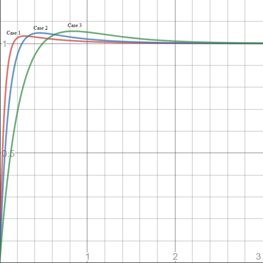
Figure 1

The plot above in figure 1 shows the output response of the PI controller where it is found that with decreasing root separation factor, the overshoot of the response is increasing and so its rise time also.

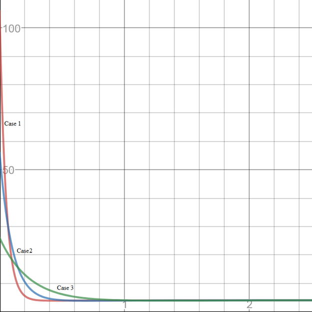
Here, in the figure 2 for the torque response of the PI controller, it is observed that with decreasing root separation factor, the peak value for the required torque decreases.

Conclusion:

The impact of root separation factor are as follows:

Case 1. For $s=-2,-20$ (Root separation factor is 10), $t_r\approx 0.15\text{seconds}$, $T_m\approx 106\text{N}\cdot \text{m}$ and $M_P\approx 1.034\text{units}$.

Case 2. For $s=-2,-10$ (Root separation factor is 5), $t_r\approx 0.25\text{seconds}$, $T_m\approx 56\text{N}\cdot \text{m}$ and $M_P\approx 1.048\text{units}$.

Case 3. For $s=-2,-4$ (Root separation factor is 2), $t_r\approx 0.49\text{seconds}$, $T_m\approx 26\text{N}\cdot \text{m}$ and $M_P\approx 1.055\text{units}$.

Thus, we see that with decrease in the root separation factor, the rise time as well as the overshoot increases. While for the required torque, the value of maximum torque decreased with increased root separation factor.