UNDERSTANDABLE STATISTICS(LL)/ACCESS
12th Edition
ISBN: 9781337805094
Author: BRASE
Publisher: CENGAGE L
bartleby

Concept explainers

bartleby

Videos

Question
Book Icon
Chapter 10.2, Problem 18P

(a)

To determine

Find the probability that the number of bacteria colonies per field.

(a)

Expert Solution
Check Mark

Answer to Problem 18P

The probability that the number of bacteria colonies per field is,

r012345 or more
P(r)0.0610.1700.2380.2220.1560.153

Explanation of Solution

Calculation:

From the given information the probability distribution of r is,

P(r)=eλλrr!

Where, λ=2.80 is the average number of bacteria colonies per field, r is the number of bacteria colonies per field.

For r=0,

The probability that there are no bacteria colonies is,

P(0)=e2.80(2.80)00!=0.061

For r=1,

The probability that there is one bacteria colony is,

P(1)=e2.80(2.80)11!=0.170

For r=2,

The probability that there are two bacteria colonies is,

P(1)=e2.80(2.80)22!=0.4772=0.238

For r=3,

The probability that there are three bacteria colonies is,

P(3)=e2.80(2.80)33!=1.3356=0.222

For r=4,

The probability that there are four bacteria colonies is,

P(4)=e2.80(2.80)44!=3.73724=0.156

For r=5 or more,

The probability that there are five or more accidents is,

P(5 or more)=1P(4or less)=1[P(0)+P(1)+P(2)+P(3)+P(4)]=1[0.061+0.170+0.238+0.222+0.156]=10.847=0.153

Hence, the probability that the number of bacteria colonies per field is,

r012345 or more
P(r)0.0610.1700.2380.2220.1560.153

(b)

To determine

Find the expected number of colonies E=100P(r) for r=0,1,2,3,4,5 or more.

(b)

Expert Solution
Check Mark

Answer to Problem 18P

The expected number of colonies is,

rExpected value
06.1
117.0
223.8
322.2
415.6
5 or more15.3

Explanation of Solution

Calculation:

For r=0,

The expected number of colonies is,

E=100P(0)=100×0.061=6.1

For r=1,

The expected number of colonies is,

E=100P(1)=100×0.170=17.0

For r=2,

The expected number of colonies is,

E=100P(2)=100×0.238=23.8

For r=3,

The expected number of colonies is,

E=100P(3)=100×0.222=22.2

For r=4,

The expected number of colonies is,

E=100P(4)=100×0.156=15.6

For r=5 or more,

The expected number of colonies is,

E=100P(5)=100×0.153=15.3

Hence, the expected number of colonies is,

rExpected value
06.1
117.0
223.8
322.2
415.6
5 or more15.3

(c)

To determine

Find the sample statistic χ2=(OE)2E.

Find the degrees of freedom.

(c)

Expert Solution
Check Mark

Answer to Problem 18P

The sample statistic is 13.116.

The degrees of freedom are 5.

Explanation of Solution

Calculation:

Test statistic:

The sample chi-square test statistic is,

χ2=(OE)2E

In the formula O is the observed frequency, E is the expected frequency, with degrees of freedom d.f.=k1, k is the number of categories,

E=(sample size n)(probability assigned to category)

The value of the chi-square statistic for the sample is,

χ2=(OE)2E=[(126.1)26.1+(1517.0)217.0+(2923.8)223.8+(1822.2)222.2+(1915.6)215.6+(715.3)215.3]=5.706+0.235+1.136+0.795+0.741+4.503=13.116

Hence, the sample statistic is 13.116.

Substitute 6 for k in the degrees of freedom formula.

d.f.=61=5

Hence, the degrees of freedom are 5.

(d)

To determine

Check whether the Poisson distribution fits the sample data or not.

(d)

Expert Solution
Check Mark

Answer to Problem 18P

There is sufficient evidence that the Poisson distribution does not fit the sample data.

Explanation of Solution

Calculation:

From the given information the value of α is 0.05, and to test the statement that the Poisson distribution fits the sample data.

The null and alternative hypothesis is,

Null hypothesis:

H0: The Poisson distribution fits the sample data.

Alternative hypothesis:

H1: The Poisson distribution does not fit the sample data.

P-value:

Step by step procedure to obtain P-value using MINITAB software is given below:

  • Choose Graph > Probability Distribution Plot choose View Probability > OK.
  • From Distribution, choose ‘Chi-Square’ distribution.
  • In Degrees of freedom, enter the value as 5.
  • Click the Shaded Area tab.
  • Choose X Value and Right Tail, for the region of the curve to shade.
  • Enter the X value as 13.116.
  • Click OK.

Output using MINITAB software is given below:

UNDERSTANDABLE STATISTICS(LL)/ACCESS, Chapter 10.2, Problem 18P

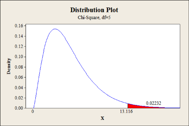
From Minitab output, the P-value is 0.0223.

Rejection rule:

  • If the P-value is less than or equal to α, then reject the null hypothesis and the test is statistically significant. That is, P-valueα.

Conclusion:

The P-value is 0.0223 and the level of significance is 0.05.

The P-value is less than the level of significance.

That is, 0.0223(=P-value)<0.05(=α).

By the rejection rule, the null hypothesis is rejected.

Hence, there is sufficient evidence that the Poisson distribution does not fit the sample data at level of significance 0.05.

Want to see more full solutions like this?

Subscribe now to access step-by-step solutions to millions of textbook problems written by subject matter experts!

Chapter 10 Solutions

UNDERSTANDABLE STATISTICS(LL)/ACCESS

Ch. 10.1 - Prob. 11PCh. 10.1 - For Problems 919, please provide the following...Ch. 10.1 - Prob. 13PCh. 10.1 - Prob. 14PCh. 10.1 - Prob. 15PCh. 10.1 - Prob. 16PCh. 10.1 - Prob. 17PCh. 10.1 - For Problems 919, please provide the following...Ch. 10.1 - Prob. 19PCh. 10.2 - Statistical Literacy For a chi-square...Ch. 10.2 - Prob. 2PCh. 10.2 - Statistical Literacy Explain why goodness-of-fit...Ch. 10.2 - Prob. 4PCh. 10.2 - For Problems 516, please provide the following...Ch. 10.2 - For Problems 516, please provide the following...Ch. 10.2 - Prob. 7PCh. 10.2 - For Problems 516, please provide the following...Ch. 10.2 - For Problems 516, please provide the following...Ch. 10.2 - For Problems 516, please provide the following...Ch. 10.2 - For Problems 516, please provide the following...Ch. 10.2 - For Problems 516, please provide the following...Ch. 10.2 - For Problems 516, please provide the following...Ch. 10.2 - Prob. 14PCh. 10.2 - Prob. 15PCh. 10.2 - Prob. 16PCh. 10.2 - Prob. 17PCh. 10.2 - Prob. 18PCh. 10.3 - Statistical Literacy Does the x distribution need...Ch. 10.3 - Critical Thinking The x distribution must be...Ch. 10.3 - Prob. 3PCh. 10.3 - For Problems 311, please provide the following...Ch. 10.3 - For Problems 311, please provide the following...Ch. 10.3 - For Problems 311, please provide the following...Ch. 10.3 - For Problems 311, please provide the following...Ch. 10.3 - For Problems 311, please provide the following...Ch. 10.3 - For Problems 311, please provide the following...Ch. 10.3 - For Problems 311, please provide the following...Ch. 10.3 - Prob. 11PCh. 10.4 - Prob. 1PCh. 10.4 - Statistical Literacy When using the F distribution...Ch. 10.4 - Prob. 3PCh. 10.4 - Prob. 4PCh. 10.4 - Prob. 5PCh. 10.4 - Prob. 6PCh. 10.4 - Prob. 7PCh. 10.4 - Prob. 8PCh. 10.4 - Prob. 9PCh. 10.4 - For Problems 512, please provide the following...Ch. 10.4 - Prob. 11PCh. 10.4 - Prob. 12PCh. 10.5 - In each problem, assume that the distributions are...Ch. 10.5 - Prob. 2PCh. 10.5 - Prob. 3PCh. 10.5 - Prob. 4PCh. 10.5 - Prob. 5PCh. 10.5 - Prob. 6PCh. 10.5 - Prob. 7PCh. 10.5 - Prob. 8PCh. 10.5 - Prob. 9PCh. 10.6 - Prob. 1PCh. 10.6 - Prob. 2PCh. 10.6 - Prob. 3PCh. 10.6 - Prob. 4PCh. 10.6 - Prob. 5PCh. 10.6 - Prob. 6PCh. 10.6 - Prob. 7PCh. 10 - Prob. 1CRPCh. 10 - Prob. 2CRPCh. 10 - Prob. 3CRPCh. 10 - Prob. 4CRPCh. 10 - Prob. 5CRPCh. 10 - Before you solve Problems 514, first classify the...Ch. 10 - Prob. 7CRPCh. 10 - Prob. 8CRPCh. 10 - Prob. 9CRPCh. 10 - Prob. 10CRPCh. 10 - Prob. 11CRPCh. 10 - Prob. 12CRPCh. 10 - Prob. 13CRPCh. 10 - Prob. 14CRPCh. 10 - Prob. 1DHCh. 10 - Prob. 1LCCh. 10 - Prob. 2LCCh. 10 - Prob. 1UTCh. 10 - Prob. 2UTCh. 10 - Prob. 3UT
Knowledge Booster
Background pattern image
Statistics
Learn more about
Need a deep-dive on the concept behind this application? Look no further. Learn more about this topic, statistics and related others by exploring similar questions and additional content below.
Similar questions
Recommended textbooks for you
Text book image
Functions and Change: A Modeling Approach to Coll...
Algebra
ISBN:9781337111348
Author:Bruce Crauder, Benny Evans, Alan Noell
Publisher:Cengage Learning
Mod-01 Lec-01 Discrete probability distributions (Part 1); Author: nptelhrd;https://www.youtube.com/watch?v=6x1pL9Yov1k;License: Standard YouTube License, CC-BY
Discrete Probability Distributions; Author: Learn Something;https://www.youtube.com/watch?v=m9U4UelWLFs;License: Standard YouTube License, CC-BY
Probability Distribution Functions (PMF, PDF, CDF); Author: zedstatistics;https://www.youtube.com/watch?v=YXLVjCKVP7U;License: Standard YouTube License, CC-BY
Discrete Distributions: Binomial, Poisson and Hypergeometric | Statistics for Data Science; Author: Dr. Bharatendra Rai;https://www.youtube.com/watch?v=lHhyy4JMigg;License: Standard Youtube License