
ELEMENTARY SATISTICS IA
13th Edition
ISBN: 9780137695522
Author: Triola
Publisher: PEARSON C
expand_more
expand_more
format_list_bulleted
Concept explainers
Videos
Textbook Question
Chapter 10.2, Problem 20BSC
Regression and Predictions. Exercises 13–28 use the same data sets as Exercises 13–28 in Section 10-1. In each case, find the regression equation, letting the first variable be the predictor (x) variable, Find the indicated predicted value by following the prediction procedure summarized in Figure 10-5 on page 493.
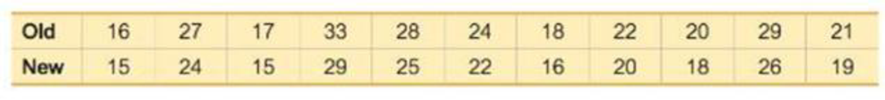
20. Revised mpg Ratings Using the listed old/new mpg ratings, find the best predicted new mpg rating for a car with an old rating of 30 mpg. Is there anything to suggest that the prediction is likely to be quite good?
Expert Solution & Answer
Want to see the full answer?
Check out a sample textbook solution
Students have asked these similar questions
Regression and Predictions. Exercises 13–28 use the same data sets as Exercises 13–28 in Section 10-1. In each case, find the regression equation, letting the first variable be the predictor (x) variable. Find the indicated predicted value by following the prediction procedure summarized in Figure 10-5 on page 493.
Old Faithful Using the listed duration and interval after times, find the best predicted “interval after” time for an eruption with a duration of 253 seconds. How does it compare to an actual eruption with a duration of 253 seconds and an interval after time of 83 minutes?
Regression and Predictions. Exercises 13–28 use the same data sets as Exercises 13–28 in Section 10-1. In each case, find the regression equation, letting the first variable be the predictor (x) variable. Find the indicated predicted value by following the prediction procedure summarized in Figure 10-5 on page 493.
Manatees Use the listed boat/manatee data. In a year not included in the data below, there were 970,000 registered pleasure boats in Florida. Find the best predicted number of manatee fatalities resulting from encounters with boats. Is the result reasonably close to 79, which was the actual number of manatee fatalities?
Q. Table provided gives data on gross domestic product (GDP) for the United States for the years 1959–2005.
a. Plot the GDP data in current and constant (i.e., 2000) dollars against time.
b. Letting Y denote GDP and X time (measured chronologically starting with 1 for 1959, 2 for 1960, through 47 for 2005), see if the following model fits the GDP data:
Yt = β1 + β2 Xt + ut
Estimate this model for both current and constant-dollar GDP.
c. How would you interpret β2?
d. If there is a difference between β2 estimated for current-dollar GDP and that estimated for constant-dollar GDP, what explains the difference?
e. From your results what can you say about the nature of inflation in the United States over the sample period?
Chapter 10 Solutions
ELEMENTARY SATISTICS IA
Ch. 10.1 - Notation Twenty different statistics students are...Ch. 10.1 - Interpreting r For the some two variables...Ch. 10.1 - Global Warming If we find that there is a linear...Ch. 10.1 - Scatterplots Match these values of r with the five...Ch. 10.1 - Bear Weight and Chest Size Fifty-four wild bears...Ch. 10.1 - Casino Size and Revenue The New York Times...Ch. 10.1 - Garbage Data Set 31 Garbage Weight in Appendix B...Ch. 10.1 - Cereal Killers The amounts of sugar (grams of...Ch. 10.1 - Explore! Exercises 9 and 10 provide two data sets...Ch. 10.1 - Explore! Exercises 9 and 10 provide two data sets...
Ch. 10.1 - Outlier Refer to the accompanying...Ch. 10.1 - Clusters Refer to the following Minitab-generated...Ch. 10.1 - Testing for a Linear Correlation. In Exercises...Ch. 10.1 - Testing for a Linear Correlation. In Exercises...Ch. 10.1 - Testing for a Linear Correlation. In Exercises...Ch. 10.1 - Testing for a Linear Correlation. In Exercises...Ch. 10.1 - Testing for a Linear Correlation. In Exercises...Ch. 10.1 - Testing for a Linear Correlation. In Exercises...Ch. 10.1 - Testing for a Linear Correlation. In Exercises...Ch. 10.1 - Testing for a Linear Correlation. In Exercises...Ch. 10.1 - Testing for a Linear Correlation. In Exercises...Ch. 10.1 - Testing for a Linear Correlation. In Exercises...Ch. 10.1 - Testing for a Linear Correlation. In Exercises...Ch. 10.1 - Testing for a Linear Correlation. In Exercises...Ch. 10.1 - Testing for a Linear Correlation. In Exercises...Ch. 10.1 - Testing for a Linear Correlation. In Exercises...Ch. 10.1 - Testing for a Linear Correlation. In Exercises...Ch. 10.1 - Testing for a Linear Correlation. In Exercises...Ch. 10.1 - Appendix B Data Sets. In Exercises 2934, use the...Ch. 10.1 - Appendix B Data Sets. In Exercises 2934, use the...Ch. 10.1 - Appendix B Data Sets. In Exercises 2934, use the...Ch. 10.1 - Appendix B Data Sets. In Exercises 2934, use the...Ch. 10.1 - Appendix B Data Sets. In Exercises 2934, use the...Ch. 10.1 - Appendix B Data Sets. In Exercises 2934, use the...Ch. 10.1 - Transformed Data In addition to testing for a...Ch. 10.1 - Finding Critical r Values Table A-6 lists critical...Ch. 10.2 - Notation Different hotels on Las Vegas Boulevard...Ch. 10.2 - Notation What is the difference between the...Ch. 10.2 - Best-Fit Line a. What is a residual? b. In what...Ch. 10.2 - Correlation and Slope What is the relationship...Ch. 10.2 - Making Predictions. In Exercises 58, let the...Ch. 10.2 - Making Predictions. In Exercises 58, let the...Ch. 10.2 - Making Predictions. In Exercises 58, let the...Ch. 10.2 - Making Predictions. In Exercises 58, let the...Ch. 10.2 - Finding the Equation of the Regression Line. In...Ch. 10.2 - Finding the Equation of the Regression Line. In...Ch. 10.2 - Effects of an Outlier Refer to the Mini...Ch. 10.2 - Effects of Clusters Refer to the Minitab-generated...Ch. 10.2 - Regression and Predictions. Exercises 1328 use the...Ch. 10.2 - Regression and Predictions. Exercises 1328 use the...Ch. 10.2 - Regression and Predictions. Exercises 1328 use the...Ch. 10.2 - Regression and Predictions. Exercises 1328 use the...Ch. 10.2 - Regression and Predictions. Exercises 1328 use the...Ch. 10.2 - Regression and Predictions. Exercises 1328 use the...Ch. 10.2 - Regression and Predictions. Exercises 1328 use the...Ch. 10.2 - Regression and Predictions. Exercises 1328 use the...Ch. 10.2 - Regression and Predictions. Exercises 1328 use the...Ch. 10.2 - Regression and Predictions. Exercises 1328 use the...Ch. 10.2 - Regression and Predictions. Exercises 1328 use the...Ch. 10.2 - Regression and Predictions. Exercises 1328 use the...Ch. 10.2 - Regression and Predictions. Exercises 13-28 use...Ch. 10.2 - Regression and Predictions. Exercises 13-28 use...Ch. 10.2 - Regression and Predictions. Exercises 13-28 use...Ch. 10.2 - Regression and Predictions. Exercises 13-28 use...Ch. 10.2 - Large Data Sets. Exercises 29-32 use the same...Ch. 10.2 - Large Data Sets. Exercises 29-32 use the same...Ch. 10.2 - Large Data Sets. Exercises 29-32 use the same...Ch. 10.2 - Large Data Sets. Exercises 29-32 use the same...Ch. 10.2 - Word Counts of Men and Women Refer to Data Set 24...Ch. 10.2 - Earthquakes Refer lo Data Set 21 Earthquakes in...Ch. 10.2 - Least-Squares Property According to the...Ch. 10.3 - se Notation Using Data Set 1 Body Data in Appendix...Ch. 10.3 - Prediction Interval Using the heights and weights...Ch. 10.3 - Coefficient of Determination Using the heights and...Ch. 10.3 - Standard Error of Estimate A random sample of 118...Ch. 10.3 - Interpreting the Coefficient of Determination. In...Ch. 10.3 - Interpreting the Coefficient of Determination. In...Ch. 10.3 - Interpreting the Coefficient of Determination. In...Ch. 10.3 - Interpreting the Coefficient of Determination. In...Ch. 10.3 - Interpreting a Computer Display. In Exercises...Ch. 10.3 - Interpreting a Computer Display. In Exercises...Ch. 10.3 - Interpreting a Computer Display. In Exercises...Ch. 10.3 - Interpreting a Computer Display. In Exercises...Ch. 10.3 - Finding a Prediction Interval. In Exercises 13-16,...Ch. 10.3 - Finding a Prediction Interval. In Exercises 13-16,...Ch. 10.3 - Finding a Prediction Interval. In Exercises 13-16,...Ch. 10.3 - Finding a Prediction Interval. In Exercises 13-16,...Ch. 10.3 - Variation and Prediction Intervals. In Exercises...Ch. 10.3 - Variation and Prediction Intervals. In Exercises...Ch. 10.3 - Variation and Prediction Intervals. In Exercises...Ch. 10.3 - Variation and Prediction Intervals. In Exercises...Ch. 10.3 - Confidence Interval for Mean Predicted Value...Ch. 10.4 - Terminology Using the lengths (in.). chest sizes...Ch. 10.4 - Best Multiple Regression Equation For the...Ch. 10.4 - Adjusted Coefficient of Determination For Exercise...Ch. 10.4 - Interpreting R2 For the multiple regression...Ch. 10.4 - Interpreting a Computer Display. In Exercises 5-8,...Ch. 10.4 - Interpreting a Computer Display. In Exercises 5-8,...Ch. 10.4 - Interpreting a Computer Display. In Exercises 5-8,...Ch. 10.4 - Interpreting a Computer Display. In Exercises 5-8,...Ch. 10.4 - City Fuel Consumption: Finding the Best Multiple...Ch. 10.4 - City Fuel Consumption: Finding the Best Multiple...Ch. 10.4 - City Fuel Consumption: Finding the Best Multiple...Ch. 10.4 - City Fuel Consumption: Finding the Best Multiple...Ch. 10.4 - Appendix B Data Sets. In Exercises 13-16, refer to...Ch. 10.4 - Prob. 14BSCCh. 10.4 - Appendix B Data Sets. In Exercises 13-16, refer to...Ch. 10.4 - Appendix B Data Sets. In Exercises 13-16, refer to...Ch. 10.4 - Testing Hypotheses About Regression Coefficients...Ch. 10.4 - Confidence Intervals for a Regression Coefficients...Ch. 10.4 - Dummy Variable Refer to Data Set 9 Bear...Ch. 10.5 - Identifying a Model and R2 Different samples are...Ch. 10.5 - Super Bowl and R2 Let x represent years coded as...Ch. 10.5 - Super Bowl and R2 Let x represent years coded as...Ch. 10.5 - Interpreting a Graph The accompanying graph plots...Ch. 10.5 - Finding the Best Model. In Exercises 5-16,...Ch. 10.5 - Finding the Best Model. In Exercises 5-16,...Ch. 10.5 - Finding the Best Model. In Exercises 5-16,...Ch. 10.5 - Finding the Best Model. In Exercises 5-16,...Ch. 10.5 - Finding the Best Model. In Exercises 5-16,...Ch. 10.5 - Finding the Best Model. In Exercises 5-16,...Ch. 10.5 - Finding the Best Model. In Exercises 5-16,...Ch. 10.5 - Finding the Best Model. In Exercises 5-16,...Ch. 10.5 - Finding the Best Model. In Exercises 5-16,...Ch. 10.5 - Finding the Best Model. In Exercises 5-16,...Ch. 10.5 - Finding the Best Model. In Exercises 5-16,...Ch. 10.5 - Finding the Best Model. In Exercises 5-16,...Ch. 10.5 - Sum of Squares Criterion In addition to the value...Ch. 10 - The following exercises are based on the following...Ch. 10 - The following exercises are based on the following...Ch. 10 - The following exercises are based on the following...Ch. 10 - The following exercises are based on the following...Ch. 10 - The following exercises are based on the following...Ch. 10 - The following exercises are based on the following...Ch. 10 - The following exercises are based on the following...Ch. 10 - The following exercises are based on the following...Ch. 10 - The following exercises are based on the following...Ch. 10 - Interpreting Scatterplot If the sample data were...Ch. 10 - Cigarette Tar and Nicotine The table below lists...Ch. 10 - 2. Cigarette Nicotine and Carbon Monoxide Refer to...Ch. 10 - Time and Motion In a physics experiment at Doane...Ch. 10 - 4. Multiple Regression with Cigarettes Use the...Ch. 10 - Stocks and Sunspots. Listed below are annual high...Ch. 10 - Stocks and Sunspots. Listed below are annual high...Ch. 10 - Stocks and Sunspots. Listed below are annual high...Ch. 10 - Stocks and Sunspots. Listed below are annual high...Ch. 10 - Stocks and Sunspots. Listed below are annual high...Ch. 10 - Cell Phones and Driving In the authors home town...Ch. 10 - Ages of Moviegoers The table below shows the...Ch. 10 - Ages of Moviegoers Based on the data from...Ch. 10 - Speed Dating Data Set 18 Speed Dating" in Appendix...Ch. 10 - Speed Dating Data Set 18 Speed Dating" in Appendix...Ch. 10 - Speed Dating Data Set 18 Speed Dating" in Appendix...Ch. 10 - Speed Dating Data Set 18 Speed Dating" in Appendix...Ch. 10 - Speed Dating Data Set 18 Speed Dating in Appendix...Ch. 10 - Speed Dating Data Set 18 Speed Dating in Appendix...Ch. 10 - Critical Thinking: Is the pain medicine Duragesic...Ch. 10 - Critical Thinking: Is the pain medicine Duragesic...Ch. 10 - Critical Thinking: Is the pain medicine Duragesic...Ch. 10 - Critical Thinking: Is the pain medicine Duragesic...Ch. 10 - Critical Thinking: Is the pain medicine Duragesic...
Knowledge Booster


Learn more about
Need a deep-dive on the concept behind this application? Look no further. Learn more about this topic, statistics and related others by exploring similar questions and additional content below.Similar questions
- Using the data in Table 6–11, calculate a 3-month moving average forecast for month 12.arrow_forwardsection 4.1 #30 In Exercises 25–30, determine whether the association between the two variables is positive or negative. Weekly ice cream sales and weekly average temperaturearrow_forwardHeart rate during laughter. Laughter is often called “the best medicine,” since studies have shown that laughter can reduce muscle tension and increase oxygenation of the blood. In the International Journal of Obesity (Jan. 2007), researchers at Vanderbilt University investigated the physiological changes that accompany laughter. Ninety subjects (18–34 years old) watched film clips designed to evoke laughter. During the laughing period, the researchers measured the heart rate (beats per minute) of each subject, with the following summary results: Mean = 73.5, Standard Deviation = 6. n=90 (we can treat this as a large sample and use z) It is well known that the mean resting heart rate of adults is 71 beats per minute. Based on the research on laughter and heart rate, we would expect subjects to have a higher heart beat rate while laughing.Construct 95% Confidence interval using z value. What is the lower bound of CI? a) Calculate the value of the test statistic.(z*) b) If…arrow_forward
- Using the data in Table 6–11, calculate a 3-month moving average forecastfor month 12.arrow_forwarda.State the predictors available in this model.arrow_forwardNational Debt The size of the total debt owed by the UnitedStates federal government continues to grow. In fact,according to the Department of the Treasury, the debt perperson living in the United States is approximately $53,000(or over $140,000 per U.S. household). The following datarepresent the U.S. debt for the years 2001–2014. Since thedebt D depends on the year y, and each input correspondsto exactly one output, the debt is a function of the year. SoD1y2 represents the debt for each year y. Source: www.treasurydirect.govDebt (billions Debt (billionsYear of dollars) Year of dollars)2001 5807 2008 10,0252002 6228 2009 11,9102003 6783 2010 13,5622004 7379 2011 14,7902005 7933 2012 16,0662006 8507 2013 16,7382007 9008 2014 17,824 (a) Plot the points 12001, 58072, 12002, 62282, and so on ina Cartesian plane.(b) Draw a line segment from the point 12001, 58072 to12006, 85072. What does the slope of this line segmentrepresent?(c) Find the average rate of change of the debt from 2002…arrow_forward
- Making Predictions. In Exercises 5–8, let the predictor variable x be the first variable given. Use the given data to find the regression equation and the best predicted value of the response variable. Be sure to follow the prediction procedure summarized in Figure 10-5 on page 493. Use a 0.05 significance level. Bear Measurements Head widths (in.) and weights (lb) were measured for 20 randomly selected bears (from Data Set 9 “Bear Measurements” in Appendix B). The 20 pairs of measurements yield x = 6.9 in., ȳ = 214.3 lb, r = 0.879, P -value = 0.000, and ŷ = −212 + 61.9x. Find the best predicted value of ŷ (weight) given a bear with a head width of 6.5 in.arrow_forwardQ1. The table provided gives data on indexes of output per hour (X) and real compensation per hour (Y) for the business and nonfarm business sectors of the U.S. economy for 1960–2005. The base year of the indexes is 1992 = 100 and the indexes are seasonally adjusted. a. Plot Y against X for the two sectors separately. b. What is the economic theory behind the relationship between the two variables? Does the scattergram support the theory? c. Estimate the OLS regression of Y on X. Note: on the table ( 1. Output refers to real gross domestic product in the sector. 2. Wages and salaries of employees plus employers’ contributions for social insurance and private benefit plans. 3. Hourly compensation divided by the consumer price index for all urban consumers for recent quarters.) Thank you!arrow_forwardInternational Visitors The number of internationalvisitors to the United States for selected years 1986–2010 is given in the table below. If you had to pick one of these models to predictthe number of international visitors in the year2020, which model would be the more reasonablechoice?arrow_forward
- City Fuel Consumption: Finding the Best Multiple Regression Equation. In Exercises 9–12, refer to the accompanying table, which was obtained using the data from 21 cars listed in Data Set 20 “Car Measurements” in Appendix B. The response (y) variable is CITY (fuel consumption in mi/gal). The predictor (x) variables are WT (weight in pounds), DISP (engine displacement in liters), and HWY (highway fuel consumption in mi /gal). If exactly two predictor (x) variables are to be used to predict the city fuel consumption, which two variables should be chosen? Why?arrow_forward(a) For United States, provide data for the variables below over the years 1993 –2007:(i) Net migration rate (per 1,000 population)(ii) Total fertility rate (live births per woman)(iii)Unemployment, general level (Thousands)(iv) Wages(v) Life expectancy at birth for both sexes combined (years)Data can be obtained from the UN database http://data.un.org/Explorer.aspxUsing R-Studio, estimate a regression equation to determine the effect of unemployment,general level, wages and life expectancy at birth for both sexes on the net migration rate.(All codes and regression output should be provided).(i) Write down the regression equation. (ii) Interpret the coefficients and determine which of the individual coefficients in theregression model are statistically significant. In responding, construct and test anyappropriate hypothesis. (iii) Interpret the coefficient of determination.arrow_forwardCity Fuel Consumption: Finding the Best Multiple Regression Equation. In Exercises 9–12, refer to the accompanying table, which was obtained using the data from 21 cars listed in Data Set 20 “Car Measurements” in Appendix B. The response (y) variable is CITY (fuel consumption in mi/gal). The predictor (x) variables are WT (weight in pounds), DISP (engine displacement in liters), and HWY (highway fuel consumption in mi /gal). Which regression equation is best for predicting city fuel consumption? Why?arrow_forward
arrow_back_ios
SEE MORE QUESTIONS
arrow_forward_ios
Recommended textbooks for you
 Calculus For The Life SciencesCalculusISBN:9780321964038Author:GREENWELL, Raymond N., RITCHEY, Nathan P., Lial, Margaret L.Publisher:Pearson Addison Wesley,
Calculus For The Life Sciences
Calculus
ISBN:9780321964038
Author:GREENWELL, Raymond N., RITCHEY, Nathan P., Lial, Margaret L.
Publisher:Pearson Addison Wesley,
Correlation Vs Regression: Difference Between them with definition & Comparison Chart; Author: Key Differences;https://www.youtube.com/watch?v=Ou2QGSJVd0U;License: Standard YouTube License, CC-BY
Correlation and Regression: Concepts with Illustrative examples; Author: LEARN & APPLY : Lean and Six Sigma;https://www.youtube.com/watch?v=xTpHD5WLuoA;License: Standard YouTube License, CC-BY