Concept explainers
Videos
Large Data Sets. Exercises 29-32 use the same Appendix B data sets as Exercises 29-32 in Section 10-1. In each case, find the regression equation, letting the first variable be the predictor (x) variable. Find the indicated predicted values following the prediction procedure summarized in Figure 10-5 on page 493.
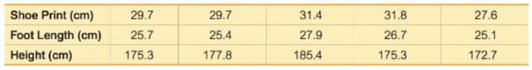
32. CSI Statistics Repeat Exercise 18 using the foot lengths and heights of the 19 males from Data Set 2 “Foot and Height.”
18. CSI Statistics Use the foot lengths and heights to find the best predicted height of a male who has a foot length of 28 cm. Would the result be helpful to police crime scene investigators in trying to describe the male?
Want to see the full answer?
Check out a sample textbook solution
Chapter 10 Solutions
Elementary Statistics, Books A La Carte Edition Plus MyLab Statistics with Pearson eText - Access Card Package (13th Edition)


- Regression and Predictions. Exercises 13–28 use the same data sets as Exercises 13–28 in Section 10-1. In each case, find the regression equation, letting the first variable be the predictor (x) variable. Find the indicated predicted value by following the prediction procedure summarized in Figure 10-5 on page 493. Internet and Nobel Laureates Find the best predicted Nobel Laureate rate for Japan, which has 79.1 Internet users per 100 people. How does it compare to Japan’s Nobel Laureate rate of 1.5 per 10 million people?arrow_forwardRegression and Predictions. Exercises 13–28 use the same data sets as Exercises 13–28 in Section 10-1. In each case, find the regression equation, letting the first variable be the predictor (x) variable. Find the indicated predicted value by following the prediction procedure summarized in Figure 10-5 on page 493. Crickets and Temperature Find the best predicted temperature at a time when a cricket chirps 3000 times in 1 minute. What is wrong with this predicted temperature?arrow_forwardChapter 9, Section 1, Exercise 006 Computer output for fitting a simple linear model is given below. State the value of the sample slope for this model and give the null and alternative hypotheses for testing if the slope in the population is different from zero. Identify the p-value and use it (and a 5% significance level) to make a clear conclusion about the effectiveness of the model.The regression equation is Y=81.0-0.0155X. Predictor Coef SE Coef T P Constant 80.96 11.62 6.97 0.000 X -0.01546 0.01288 -1.20 0.245arrow_forward
- A box office analyst seeks to predict opening weekend box office gross for movies. Toward this goal, the analyst plans to use online trailer views as a predictor. For each of the 66 movies, the number of online trailer views from the release of the trailer through the Saturday before a movie opens and the opening weekend box office gross (in millions of dollars) are collected and stored in the accompanying table. The least-squares regression equation for these data is Yi=−1.068+1.394Xi and the standard error of the estimate is SYX=19.412. Assume that the straight-line model is appropriate and there are no serious violations the assumptions of the least-squares regression model. Significance level at 0.05 . Complete parts (a) and (b) below.arrow_forwardA box office analyst seeks to predict opening weekend box office gross for movies. Toward this goal, the analyst plans to use online trailer views as a predictor. For each of the 66 movies, the number of online trailer views from the release of the trailer through the Saturday before a movie opens and the opening weekend box office gross (in millions of dollars) are collected and stored in the accompanying table. The least-squares regression equation for these data is Yi=−1.606+1.428Xi and the standard error of the estimate is SYX=19.348. Assume that the straight-line model is appropriate and there are no serious violations the assumptions of the least-squares regression model. Complete parts (a) and (b) below. a. At the 0.01 level of significance, is there evidence of a linear relationship between online trailer views and opening weekend box office gross? Determine the hypotheses for the test. b. Construct a 95%confidence interval estimate of the population…arrow_forwardRegression and Predictions. Exercises 13–28 use the same data sets as Exercises 13–28 in Section 10-1. In each case, find the regression equation, letting the first variable be the predictor (x) variable. Find the indicated predicted value by following the prediction procedure summarized in Figure 10-5 on page 493. Old Faithful Using the listed duration and interval after times, find the best predicted “interval after” time for an eruption with a duration of 253 seconds. How does it compare to an actual eruption with a duration of 253 seconds and an interval after time of 83 minutes?arrow_forward
- Cinema HD an online movie streaming service that offers a wide variety of award-winning TV shows, movies, animes, and documentaries, would like to determine the mathematical trend of memberships in order to project future needs. Year 2013 2014 2015 2016 2017 2018 2019 2020 2021 Membership 17 16 16 21 20 20 23 25 24 Use the following time series data, to develop a regression equation relating memberships to time. Forecast 2023 membership Assuming the COVID-19 pandemic comes to an end in 2021, in your opinion, how will this affect membership? Why? How will this affect your prediction? What are the issues associated with qualitative forecasting, and how are these overcome? Provide an example of qualitative forecasting and explain the shortcomings.arrow_forwardA box office analyst seeks to predict opening weekend box office gross for movies. Toward this goal, the analyst plans to use online trailer views as a predictor. For each of the 66 movies, the number of online trailer views from the release of the trailer through the Saturday before a movie opens and the opening weekend box office gross (in millions of dollars) are collected and stored in the accompanying table. The least-squares regression equation for these data isYi=−0.914+1.408Xi and the standard error of the estimate is SYX=19.887. Assume that the straight-line model is appropriate and there are no serious violations the assumptions of the least-squares regression model. Compute the test statistic.arrow_forwardConsider the delivery time data discussed in Example 11.3 .a. Develop a regression model using the prediction data set. b. How do the estimates of the parameters in this model compare with those from the model developed from the estimation data? What does this imply about model validity? c. Use the model developed in part a to predict the delivery times for the observations in the original estimation data. Are your results consistent with those obtained in Example 11.3 ?arrow_forward
- A box office analyst seeks to predict opening weekend box office gross for movies. Toward this goal, the analyst plans to use online trailer views as a predictor. For each of the 66 movies, the number of online trailer views from the release of the trailer through the Saturday before a movie opens and the opening weekend box office gross (in millions of dollars) are collected and stored in the accompanying table. The least-squares regression equation for these data is Yi=−1.660+1.417Xi and the standard error of the estimate is SYX=19.349. Assume that the straight-line model is appropriate and there are no serious violations the assumptions of the least-squares regression model.arrow_forwardMovieflix, an online movie streaming service that offers a wide variety of award-winning TV shows, movies, animes, and documentaries, would like to determine the mathematical trend of memberships in order to project future needs. Year 2013 2014 2015 2016 2017 2018 2019 2020 2021 Membership 17 16 16 21 20 20 23 25 24 Use the following time series data, to develop a regression equation relating memberships to time. Forecast 2023 membership Assuming the COVID-19 pandemic comes to an end in 2021, in your opinion, how will this affect membership? Why? How will this affect your prediction?arrow_forward9. A wildlife researcher is interested in predicting an alligator’s weight (in pounds) based on its length (in inches). Data was obtained from a large random sample of alligators, and the regression equation turned out as follows: Predicted weight = –393 + 5.9 (length) Which one of the following statements is a correct interpretation of this equation? 1. As weight increases by one pound, length is predicted to decrease by 393 inches. 2. As length increases by one inch, weight is predicted to increase by 5.9 pounds. 3. As weight increases by one pound, length is predicted to increase by 5.9 inches. 4. As length increases by one inch, weight is predicted to decrease by 393 pounds. 5. Approximately 5.9% of the variability in weight can be explained by the regression equation.arrow_forward
 College AlgebraAlgebraISBN:9781305115545Author:James Stewart, Lothar Redlin, Saleem WatsonPublisher:Cengage Learning
 Linear Algebra: A Modern IntroductionAlgebraISBN:9781285463247Author:David PoolePublisher:Cengage Learning