Chapter 10.3, Problem 26E

Samples of six different brands of diet/imitation margarine were analyzed to determine the level of physiologically active polyunsaturated fatty acids (PAPFUA, in percentages), resulting in the following data:

Imperial	14.1	13.6	14.4	14.3
Parkay	12.8	12.5	13.4	13.0	12.3
Blue Bonnet	13.5	13.4	14.1	14.3
Chiffon	13.2	12.7	12.6	13.9
Mazola	16.8	17.2	16.4	17.3	18.0
Fleischmann 's	18.1	17.2	18.7	18.4

(The preceding numbers are fictitious, but the sample means agree with data reported in the January 1975 issue of Consumer Reports.)

a. Use ANOVA to test for differences among the true average PAPFUA percentages for the different brands.

b. Compute CIs for all (µ_i − µ_j)’s.

c. Mazola and Fleischmann’s are corn-based, whereas the others are soybean-based. Compute a CI for

     $\frac{\left({\mu }_1+{\mu }_2+{\mu }_3+{\mu }_4\right)}{4}-\frac{\left({\mu }_5+{\mu }_6\right)}{2}s$

[Hint: Modify the expression for $V\left(\hat{\theta }\right)$ that led to (10.5) in the previous section.]

To determine

Test for differences among the true average PAPFUA percentages for the brands, using ANOVA.

Answer to Problem 26E

The test using ANOVA suggests that there is significant difference among the true average PAPFUA percentages for the brands, at level of significance 0.01.

Explanation of Solution

Given info:

The data gives the observations on percentages of physically active polyunsaturated fatty acids (PAPFUA) in specimens of 6 brands of diet/imitation margarine, namely, Imperial, Parkay, Blue Bonnet, Chiffon, Mazola and Fleischmann’s.

Calculation:

Suppose there are I treatments and $J_i$ observations corresponding to the i^th treatment in a designed experiment. Then, the following properties hold true:

• Degrees of freedom (df): The treatment df is $I-1$, the total df is $n-1={\displaystyle \sum _i{J}_i}-1$. The error df is the difference between these, that is, $n-I={\displaystyle \sum _i\left(J_i-1\right)}$.
• Sum of squares: The total sum of squares (SST), treatment sum of squares (SSTr) and error sum of squares (SSE) are related as: $\text{SST}=\text{SSTr}+\text{SSE}$.
• Mean of squares: The mean of squares is the ratio of the sum of squares to the corresponding df. The mean square error (MSE) is, $\text{MSE}=\frac{\text{SSE}}{n-I}$. The mean square treatment (MSTr) is, $\text{MSTr}=\frac{\text{SSTr}}{I-1}$.
• The F-statistic: The F- statistic is the ratio of MSTr and MSE, that is, $F=\frac{\text{MSTr}}{\text{MSE}}$.

Here, each brand is a treatment. The brands are numbered respectively 1 to 6.

Denote $X_{ij}$ as the j^th observation corresponding to the i^th treatment, for each $i=1,2,\mathrm{...},I\left(=6\right)$.

State the test hypotheses.

Null hypothesis:

$H_0:{\mu }_1={\mu }_2={\mu }_3={\mu }_4={\mu }_5={\mu }_6=0$

That is, the effects of all the treatments are similar.

Alternative hypothesis:

$H_a:{\mu }_i\ne 0$, for at least one $i=1,2,3,4,5,6$.

That is, the effects of all the treatments are not similar.

Test statistic:

The suitable test statistic is the F- statistic, which is the ratio of the mean square treatment (MSTr) and the mean square error (MSE), that is,

$F=\frac{\text{MSTr}}{\text{MSE}}$.

Degrees of freedom:

In this case, number of treatments is $I=6$. Thus, the treatment df is:

$\begin{array}{c}I-1=6-1\\ =5.\end{array}$

The total df is:

$\begin{array}{c}n-1={\displaystyle \sum _{i=1}^I{J}_i}-1\\ =\left(4+5+4+4+5+4\right)-1\\ =26-1\\ =25.\end{array}$

The error df is:

$\begin{array}{c}n-I=26-6\\ =20.\end{array}$

The numerator degrees of freedom is:

$\begin{array}{c}{\nu }_1=I-1\\ =5.\end{array}$

The denominator degrees of freedom is:

$\begin{array}{c}{\nu }_2=n-I\\ =20.\end{array}$

Calculation for test statistic:

The sample total corresponding to the i^th treatment is:

$X_{i.}={\displaystyle \sum _{j=1}^{J_i}{X}_{ij}},i=1,2,\mathrm{...},I$.

The sample mean corresponding to the i^th treatment is:

${\overline{X}}_{i.}=\frac{1}{J_i}{\displaystyle \sum _{j=1}^{J_i}{X}_{ij}},i=1,2,\mathrm{...},I$.

The calculation for the means of the 4 treatments is shown in the following table:

Treatment 1	Treatment 2	Treatment 3	Treatment 4	Treatment 5	Treatment 6
14.1	12.8	13.5	13.2	16.8	18.1
13.6	12.5	13.4	12.7	17.2	17.2
14.4	13.4	14.1	12.6	16.4	18.7
14.3	13	14.3	13.9	17.3	18.4
	12.3			18
$J_1=4$	$J_2=5$	$J_3=4$	$J_4=4$	$J_5=5$	$J_6=4$
$X_{1.}=56.4$	$X_{2.}=64.0$	$X_{3.}=55.3$	$X_{4.}=52.4$	$X_{5.}=85.7$	$X_{6.}=72.4$
${\overline{X}}_{1.}=14.10$	${\overline{X}}_{2.}=12.80$	${\overline{X}}_{3.}=13.82$	${\overline{X}}_{4.}=13.10$	${\overline{X}}_{5.}=17.14$	${\overline{X}}_{6.}=18.10$

The grand total is:

$\begin{array}{c}{X}_{\cdot \cdot }={\displaystyle \sum _{i=1}^I{\displaystyle \sum _{J=1}^{J_i}{X}_{ij}}}\\ ={\displaystyle \sum _{i=1}^I{X}_{i.}}\\ =56.4+64.0+55.3+52.4+85.7+72.4\\ =\mathrm{386.2.}\end{array}$.

Thus, the grand mean is:

$\begin{array}{c}\overline{X}\mathrm{..}=\frac{1}{n}{X}_{\mathrm{..}}\\ =\frac{386.2}{26}\\ =\mathrm{14.85.}\end{array}$

The sum of squares of treatments, SSTr is:

$\begin{array}{c}\text{SSTr}={\displaystyle \sum _{i=1}^I\frac{1}{J_i}{X}_{i.}^2}-\frac{1}{n}{X}_{\mathrm{..}}^2\\ =\left[\frac{{\left(56.4\right)}^2}{4}+\frac{{\left(64.0\right)}^2}{5}+\frac{{\left(55.3\right)}^2}{4}+\frac{{\left(52.4\right)}^2}{4}+\frac{{\left(85.7\right)}^2}{5}+\frac{{\left(72.4\right)}^2}{4}\right]-\frac{{\left(386.2\right)}^2}{26}\\ =\frac{3,180.96}{4}+\frac{4,096.00}{5}+\frac{3,058.09}{4}+\frac{2,745.76}{4}+\frac{7,344.49}{5}+\frac{5,241.76}{4}-\frac{149,150.4}{26}\\ =795.24+819.20+764.52+686.44+1,468.90+1,310.44-5,736.56\end{array}$

$=108.18$.

Thus, the mean square of treatments, MSTr is:

$\begin{array}{c}\text{MSTr}=\frac{\text{SSTr}}{I-1}\\ =\frac{108.18}{5}\\ =\mathrm{21.636.}\end{array}$

The total sum of squares, SST is:

$\text{SST}={\displaystyle \sum _{i=1}^I{\displaystyle \sum _{j=1}^{J_i}{X}_{ij}{}^2}}-\frac{1}{n}{X}^2{}_{\cdot \cdot }$

The calculation for ${\displaystyle \sum _{j=1}^J{X}_{ij}{}^2}$ is shown in the following table:

Brand 1	$X_{1j}$	14.1	13.6	14.4	14.3		$\begin{array}{l}{\displaystyle \sum _{j=1}^{J_1}{X}_{1j}{}^2}\\ =795.62\end{array}$
	$X^2{}_{1j}$	198.81	184.96	207.36	204.49
Brand 2	$X_{2j}$	12.8	12.5	13.4	13	12.3	$\begin{array}{l}{\displaystyle \sum _{j=1}^{J_2}{X}_{2j}{}^2}\\ =819.94\end{array}$
	$X^2{}_{2j}$	163.84	156.25	179.56	169	151.29
Brand 3	$X_{3j}$	13.5	13.4	14.1	14.3		$\begin{array}{l}{\displaystyle \sum _{j=1}^{J_3}{X}_{3j}{}^2}\\ =765.11\end{array}$
	$X^2{}_{3j}$	182.25	179.56	198.81	204.49
Brand 4	$X_{4j}$	13.2	12.7	12.6	13.9		$\begin{array}{l}{\displaystyle \sum _{j=1}^{J_4}{X}_{4j}{}^2}\\ =687.5\end{array}$
	$X^2{}_{4j}$	174.24	161.29	158.76	193.21
Brand 5	$X_{5j}$	16.8	17.2	16.4	17.3	18	$\begin{array}{l}{\displaystyle \sum _{j=1}^{J_5}{X}_{5j}{}^2}\\ =1,470.33\end{array}$
	$X^2{}_{5j}$	282.24	295.84	268.96	299.29	324
Brand 6	$X_{6j}$	18.1	17.2	18.7	18.4		$\begin{array}{l}{\displaystyle \sum _{j=1}^{J_6}{X}_{6j}{}^2}\\ =1,311.70\end{array}$
	$X^2{}_{6j}$	327.61	295.84	349.69	338.56

Thus,

$\begin{array}{c}\text{SST}={\displaystyle \sum _{i=1}^I{\displaystyle \sum _{j=1}^{J_i}{X}_{ij}{}^2}}-\frac{1}{n}{X}^2{}_{\cdot \cdot }\\ =\left(795.62+819.94+765.11+687.50+1,470.33+1,311.70\right)-5,736.56\\ =\mathrm{113.64.}\end{array}$

Now,

$\text{SST}=\text{SSTr}+\text{SSE}$.

Thus,

$\begin{array}{c}\text{SSE}=\text{SST}-\text{SSTr}\\ =113.64-108.18\\ =\mathrm{5.46.}\end{array}$

As a result,

$\begin{array}{c}\text{MSE}=\frac{\text{SSE}}{n-I}\\ =\frac{5.46}{20}\\ =\mathrm{0.273.}\end{array}$

Thus, the F-statistic is:

$\begin{array}{c}F=\frac{\text{MSTr}}{\text{MSE}}\\ =\frac{21.636}{0.273}\\ =\mathrm{79.25.}\end{array}$

Level of significance:

Assume that the level of significance here is $\alpha =0.01$.

Critical value:

The critical value for the $F_{{\nu }_1,{\nu }_2}$ distribution at level of significance $\alpha$ is $F_{\alpha ;{\nu }_1,{\nu }_2}$, which is the value of the $F_{{\nu }_1,{\nu }_2}$-distribution, the probability above which is $\alpha$.

Here, the critical value would be $F_{0.01;5,20}$. From the Table A.9, “Critical Values for F Distributions”, $F_{0.01;5,20}=4.10$.

P-value:

The P-value is the area to the right of the F-statistic value f, under the $F_{{\nu }_1,{\nu }_2}$ distribution curve, that is, $P\text{-value}=P\left(F_{{\nu }_1,{\nu }_2}>f\right)$

Hence, the P-value is $P\text{-value}=P\left(F_{5,20}>79.25\right)$.

Here, the test statistic value, $f=79.25$, which is higher than the critical value 4.10 corresponding to $F_{0.01;5,20}$.

That is, $F_{0.01;5,20}\left(=4.10\right)<f\left(=79.25\right)$.

Rejection rule:

If the P-value is less than the level of significance $\alpha$, such that $P\text{-value}<\alpha$, then reject the null hypothesis at level $\alpha$.

Conclusion:

Here, the P-value is less than the significance level 0.01.

That is, $P\text{-value}<0.01$.

Thus, the decision is “reject the null hypothesis”.

Therefore, the data provide sufficient evidence to conclude that the effects of all the treatments are not similar.

Thus, the test using ANOVA suggests that there is significant difference among the true average PAPFUA percentages for the brands, at level of significance 0.01.

To determine

Compute CI’s for each $\left({\mu }_i-{\mu }_j\right)$.

Answer to Problem 26E

The CI’s (confidence intervals) for each $\left({\mu }_i-{\mu }_j\right)$ are:

Pair	Confidence interval
1,2	(–0.07, 2.67)
1,3	(–1.16, 1.72)
1,4	(–0.44, 2.44)
1,5	(–4.41, –1.67)
1,6	(–5.44, –2.56)
2,3	(–2.39, 0.35)
2,4	(–1.67, 1.07)
2,5	(–5.63, –3.05)
2,6	(–6.67, –3.93)
3,4	(–0.74, 2.14)
3,5	(–4.69, –1.95)
3,6	(–5.72, –2.84)
4,5	(–5.41, –2.67)
4,6	(–6.44, –3.56)
5,6	(–2.33, 0.41)

Explanation of Solution

Calculation:

The confidence interval for each pair of means, $\left({\mu }_i-{\mu }_j\right)$ is given as:

${\overline{X}}_{i.}-{\overline{X}}_{j.}-w_{ij}\le {\mu }_i-{\mu }_j\le {\overline{X}}_{i.}-{\overline{X}}_{j.}+w_{ij}$.

Here, $w_{ij}=Q_{\alpha ,I,n-I}\cdot \sqrt{\frac{\text{MSE}}{2}\left(\frac{1}{J_i}+\frac{1}{J_j}\right)}$ and $Q_{\alpha ,I,n-I}$ is the Studentized range statistic.

The study contains $I=6$ treatments. Thus, total number of pairs of $\left({\mu }_i-{\mu }_j\right)$ available is $15\left[=\left(\begin{array}{l}6\\ 2\end{array}\right)\right]$.

From Table A.10 “Critical Values for Studentized Range Distribution”, $Q_{0.01;6,20}=5.51$.

It is known that $\frac{1}{J_i}+\frac{1}{J_j}=\frac{1}{J_j}+\frac{1}{J_i}$. As a result, the subscript ‘i’ and ‘j’ can be used interchangeably.

Thus, for treatment pairs $\left(1,2\right)$, $\left(1,5\right)$, $\left(2,3\right)$, $\left(2,4\right)$, $\left(2,6\right)$, $\left(3,5\right)$, $\left(4,5\right)$ and $\left(5,6\right)$ $J_i=4$, $J_j=5$.

In that case, the value of w is,

$\begin{array}{c}{w}_{ij}=Q_{\alpha ,I,n-I}\cdot \sqrt{\frac{\text{MSE}}{2}\left(\frac{1}{J_i}+\frac{1}{J_j}\right)}\\ =5.51\times \sqrt{\frac{0.273}{2}\left(\frac{1}{4}+\frac{1}{5}\right)}\\ =5.51\times \sqrt{0.1365\times \frac{9}{35}}\\ =5.51\times 0.2478\end{array}$

$\approx 1.37$.

For treatment pairs $\left(1,3\right)$, $\left(1,4\right)$, $\left(1,6\right)$, $\left(3,4\right)$, $\left(3,6\right)$, $\left(4,6\right)$ $J_i=4$, $J_j=4$.

In that case, the value of w is,

$\begin{array}{c}{w}_{ij}=Q_{\alpha ,I,n-I}\cdot \sqrt{\frac{\text{MSE}}{2}\left(\frac{1}{J_i}+\frac{1}{J_j}\right)}\\ =5.51\times \sqrt{0.1365\left(\frac{1}{4}+\frac{1}{4}\right)}\\ =5.51\times \sqrt{0.1365\times \frac{1}{2}}\\ =5.51\times 0.2612\end{array}$

$\approx 1.44$.

For treatment pair $\left(2,5\right)$, $J_i=5$, $J_j=5$.

In that case, the value of w is,

$\begin{array}{c}{w}_{ij}=Q_{\alpha ,I,n-I}\cdot \sqrt{\frac{\text{MSE}}{2}\left(\frac{1}{J_i}+\frac{1}{J_j}\right)}\\ =5.51\times \sqrt{0.1365\left(\frac{1}{5}+\frac{1}{5}\right)}\\ =5.51\times \sqrt{0.1365\times \frac{2}{5}}\\ =5.51\times 0.2337\end{array}$

$\approx 1.29$.

The calculations for the confidence intervals are shown in the following table:

Pair	${\overline{X}}_{i.},{\overline{X}}_{j.}$	${\overline{X}}_{i.}-{\overline{X}}_{j.}$	$w_{ij}$	${\overline{X}}_{i.}-{\overline{X}}_{j.}-w_{ij}$	${\overline{X}}_{i.}-{\overline{X}}_{j.}+w_{ij}$	$\left(\begin{array}{l}{\overline{X}}_{i.}-{\overline{X}}_{j.}-w_{ij},\\ {\overline{X}}_{i.}-{\overline{X}}_{j.}+w_{ij}\end{array}\right)$
1,2	14.10, 12.80	1.30	1.37	–0.07	2.67	(–0.07, 2.67)
1,3	14.10, 13.82	0.28	1.44	–1.16	1.72	(–1.16, 1.72)
1,4	14.10, 13.10	1.00	1.44	–0.44	2.44	(–0.44, 2.44)
1,5	14.10, 17.14	–3.04	1.37	–4.41	–1.67	(–4.41, –1.67)
1,6	14.10, 18.10	–4.00	1.44	–5.44	–2.56	(–5.44, –2.56)
2,3	12.80, 13.82	–1.02	1.37	–2.39	0.35	(–2.39, 0.35)
2,4	12.80, 13.10	–0.30	1.37	–1.67	1.07	(–1.67, 1.07)
2,5	12.80, 17.14	–4.34	1.29	–5.63	–3.05	(–5.63, –3.05)
2,6	12.80, 18.10	–5.30	1.37	–6.67	–3.93	(–6.67, –3.93)
3,4	13.80, 13.10	0.70	1.44	–0.74	2.14	(–0.74, 2.14)
3,5	13.82, 17.14	–3.32	1.37	–4.69	–1.95	(–4.69, –1.95)
3,6	13.82, 18.10	–4.28	1.44	–5.72	–2.84	(–5.72, –2.84)
4,5	13.10, 17.14	–4.04	1.37	–5.41	–2.67	(–5.41, –2.67)
4,6	13.10, 18.10	–5.00	1.44	–6.44	–3.56	(–6.44, –3.56)
5,6	17.14, 18.10	–0.96	1.37	–2.33	0.41	(–2.33, 0.41)

To determine

Find a CI for $\frac{\left({\mu }_1+{\mu }_2+{\mu }_3+{\mu }_4\right)}{4}-\frac{\left({\mu }_5+{\mu }_6\right)}{2}$.

Answer to Problem 26E

The CI (confidence interval) for $\frac{\left({\mu }_1+{\mu }_2+{\mu }_3+{\mu }_4\right)}{4}-\frac{\left({\mu }_5+{\mu }_6\right)}{2}$ is $\underset{\_}{\left(-4.7849,-3.5451\right)}$.

Explanation of Solution

Given info:

The brands Mazola and Fleischmann’s produce corn-based diet/imitation margarine, whereas the others produce soybean based ones.

Calculation:

Confidence interval for parametric functions:

The $100\left(1-\alpha \right)\%$ confidence interval for a function of ${\mu }_i$’s, $\theta ={\displaystyle \sum _i{c}_i{\mu }_i}$, where $c_i$’s are constants for $i=1,2,\mathrm{...},I$, is given as:

${\displaystyle \sum _i{c}_i{\overline{x}}_i}\pm t_{\frac{\alpha }{2},N-I}\sqrt{\text{MSE}{\displaystyle \sum _i\frac{c_i^2}{J_i}}}$.

Given that,

$\begin{array}{c}\theta =\frac{\left({\mu }_1+{\mu }_2+{\mu }_3+{\mu }_4\right)}{4}-\frac{\left({\mu }_5+{\mu }_6\right)}{2}\\ =\frac{1}{4}{\mu }_1+\frac{1}{4}{\mu }_2+\frac{1}{4}{\mu }_3+\frac{1}{4}{\mu }_4-\frac{1}{2}{\mu }_5-\frac{1}{2}{\mu }_6\\ =0.25{\mu }_1+0.25{\mu }_2+0.25{\mu }_3+0.25{\mu }_4-0.5{\mu }_5-0.5{\mu }_6.\end{array}$

Compare this for the general expression $\theta ={\displaystyle \sum _i{c}_i{\mu }_i}$. Thus, here, $c_1=c_2=c_3=c_4=0.25$ and $c_5=c_6=-0.5$.

As a result,

$\begin{array}{c}{\displaystyle \sum _i\frac{c_i^2}{J_i}}=\frac{{\left(0.25\right)}^2}{4}+\frac{{\left(0.25\right)}^2}{5}+\frac{{\left(0.25\right)}^2}{4}+\frac{{\left(0.25\right)}^2}{4}+\frac{{\left(-0.5\right)}^2}{5}+\frac{{\left(-0.5\right)}^2}{4}\\ =0.0625+0.0625+0.0625+0.0625+0.25+0.25\\ =0.015625+0.0125+0.015625+0.015625+0.05+0.0625\\ \approx \mathrm{0.172.}\end{array}$

Use the available values ${\overline{X}}_{1.}=14.10$, ${\overline{X}}_{2.}=12.80$, ${\overline{X}}_{3.}=13.82$, ${\overline{X}}_{4.}=13.10$, ${\overline{X}}_{5.}=17.14$ and ${\overline{X}}_{6.}=18.10$ to compute ${\displaystyle \sum _i{c}_i{\overline{x}}_i}$:

$\begin{array}{c}{\displaystyle \sum _i{c}_i{\overline{x}}_i}=\left(0.25\times 14.10\right)+\left(0.25\times 12.80\right)+\left(0.25\times 13.82\right)\\ +\left(0.25\times 13.10\right)+\left(\left(-0.5\right)\times 17.14\right)+\left(\left(-0.5\right)\times 18.10\right)\\ =3.525+3.2+3.455+3.275-8.57-9.05\\ =-\mathrm{4.165.}\end{array}$

Here, the level of significance is $\alpha =0.01$. As a result,

$\begin{array}{c}\frac{\alpha }{2}=\frac{0.01}{2}\\ =\mathrm{0.005.}\end{array}$

Thus, $t_{\frac{\alpha }{2};n-I}=t_{0.025,20}$.

Critical value:

Software procedure:

Step by step procedure to the critical value using MINITAB software is given as,

• Choose Graph > Probability Distribution Plot > View Probability.
• In Distribution, select t and in Degrees of freedom enter 20.
• Go to Shaded Area, select Probability and Right Tail, enter probability value as 0.005.
• Click OK.

Output using MINITAB software is given as,

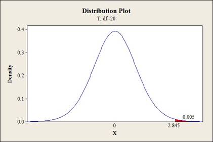
From the output, $t_{0.025,20}=2.845$.

Substitute the values in the expression for the confidence interval (CI):

$\begin{array}{c}{\displaystyle \sum _i{c}_i{\overline{x}}_i}\pm t_{\frac{\alpha }{2},N-I}\sqrt{\text{MSE}{\displaystyle \sum _i\frac{c_i^2}{J_i}}}=-4.165\pm \left[2.845\times \sqrt{0.276\times 0.172}\right]\\ =-4.165\pm \left[2.845\times \sqrt{0.047472}\right]\\ =-4.165\pm \left[2.845\times 0.2179\right]\\ =-4.165\pm 0.6199\end{array}$

        $\begin{array}{c}=\left(-4.165-0.6199,-4.165+0.6199\right)\\ =\underset{\_}{\left(-4.7849,-3.5451\right)}.\end{array}$

Thus, the CI (confidence interval) for $\frac{\left({\mu }_1+{\mu }_2+{\mu }_3+{\mu }_4\right)}{4}-\frac{\left({\mu }_5+{\mu }_6\right)}{2}$ is $\underset{\_}{\left(-4.7849,-3.5451\right)}$.