ELEMENTARY STATISTICS-W/ACCESS >CUSTOM<
3rd Edition
ISBN: 9781323594889
Author: Triola
Publisher: PEARSON C
expand_more
expand_more
format_list_bulleted
Concept explainers
Videos
Textbook Question
Chapter 10.4, Problem 10BSC
City Fuel Consumption: Finding the Best Multiple Regression Equation. In Exercises 9-12, refer to the accompanying table, which was obtained using the data from 21 cars listed in Data Set 20 “Car Measurements" in Appendix B. The response (y) variable is CITY (fuel consumption in mi/gal). The predictor (x) variables are WT (weight in pounds), DISP (engine displacement in liters), and HWY (highway fuel consumption in mi/gal).
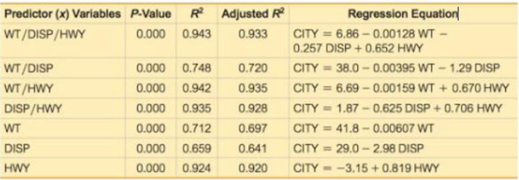
10. If exactly two predictor (x) variables are to be used to predict the city fuel consumption, which two variables should be chosen? Why?
Expert Solution & Answer
Want to see the full answer?
Check out a sample textbook solution
Students have asked these similar questions
Demand Estimation for The San Francisco Bread Company
Consider the hypothetical example of The San Francisco Bread Company, a San Francisco-based chain of bakery/cafes. San Francisco Bread Company has initiated an empirical estimation of customer traffic at 30 regional locations to help the firm formulate pricing and promotional plans for the coming year. Annual operating data for the 30 outlets appear in the attached Table 1.
The following regression equation was fit to these data:
Qi = b0 + b1Pi + b2Pxi + b3Adi + b4Ii + uit.
Where: Q is the number of meals served,
P is the average price per meal (customer ticket amount, in dollars),
Px is the average price charged by competitors (in dollars),
Ad is the local advertising budget for each outlet (in dollars),
I is the average income per household in each outlet’s service area,
ui…
Chapter 10 Solutions
ELEMENTARY STATISTICS-W/ACCESS >CUSTOM<
Ch. 10.1 - Notation Twenty different statistics students are...Ch. 10.1 - Interpreting r For the some two variables...Ch. 10.1 - Global Warming If we find that there is a linear...Ch. 10.1 - Scatterplots Match these values of r with the five...Ch. 10.1 - Bear Weight and Chest Size Fifty-four wild bears...Ch. 10.1 - Casino Size and Revenue The New York Times...Ch. 10.1 - Garbage Data Set 31 Garbage Weight in Appendix B...Ch. 10.1 - Cereal Killers The amounts of sugar (grams of...Ch. 10.1 - Explore! Exercises 9 and 10 provide two data sets...Ch. 10.1 - Explore! Exercises 9 and 10 provide two data sets...
Ch. 10.1 - Outlier Refer to the accompanying...Ch. 10.1 - Clusters Refer to the following Minitab-generated...Ch. 10.1 - Testing for a Linear Correlation. In Exercises...Ch. 10.1 - Testing for a Linear Correlation. In Exercises...Ch. 10.1 - Testing for a Linear Correlation. In Exercises...Ch. 10.1 - Testing for a Linear Correlation. In Exercises...Ch. 10.1 - Testing for a Linear Correlation. In Exercises...Ch. 10.1 - Testing for a Linear Correlation. In Exercises...Ch. 10.1 - Testing for a Linear Correlation. In Exercises...Ch. 10.1 - Testing for a Linear Correlation. In Exercises...Ch. 10.1 - Testing for a Linear Correlation. In Exercises...Ch. 10.1 - Testing for a Linear Correlation. In Exercises...Ch. 10.1 - Testing for a Linear Correlation. In Exercises...Ch. 10.1 - Testing for a Linear Correlation. In Exercises...Ch. 10.1 - Testing for a Linear Correlation. In Exercises...Ch. 10.1 - Testing for a Linear Correlation. In Exercises...Ch. 10.1 - Testing for a Linear Correlation. In Exercises...Ch. 10.1 - Testing for a Linear Correlation. In Exercises...Ch. 10.1 - Appendix B Data Sets. In Exercises 2934, use the...Ch. 10.1 - Appendix B Data Sets. In Exercises 2934, use the...Ch. 10.1 - Appendix B Data Sets. In Exercises 2934, use the...Ch. 10.1 - Appendix B Data Sets. In Exercises 2934, use the...Ch. 10.1 - Appendix B Data Sets. In Exercises 2934, use the...Ch. 10.1 - Appendix B Data Sets. In Exercises 2934, use the...Ch. 10.1 - Transformed Data In addition to testing for a...Ch. 10.1 - Finding Critical r Values Table A-6 lists critical...Ch. 10.2 - Notation Different hotels on Las Vegas Boulevard...Ch. 10.2 - Notation What is the difference between the...Ch. 10.2 - Best-Fit Line a. What is a residual? b. In what...Ch. 10.2 - Correlation and Slope What is the relationship...Ch. 10.2 - Making Predictions. In Exercises 58, let the...Ch. 10.2 - Making Predictions. In Exercises 58, let the...Ch. 10.2 - Making Predictions. In Exercises 58, let the...Ch. 10.2 - Making Predictions. In Exercises 58, let the...Ch. 10.2 - Finding the Equation of the Regression Line. In...Ch. 10.2 - Finding the Equation of the Regression Line. In...Ch. 10.2 - Effects of an Outlier Refer to the Mini...Ch. 10.2 - Effects of Clusters Refer to the Minitab-generated...Ch. 10.2 - Regression and Predictions. Exercises 1328 use the...Ch. 10.2 - Regression and Predictions. Exercises 1328 use the...Ch. 10.2 - Regression and Predictions. Exercises 1328 use the...Ch. 10.2 - Regression and Predictions. Exercises 1328 use the...Ch. 10.2 - Regression and Predictions. Exercises 1328 use the...Ch. 10.2 - Regression and Predictions. Exercises 1328 use the...Ch. 10.2 - Regression and Predictions. Exercises 1328 use the...Ch. 10.2 - Regression and Predictions. Exercises 1328 use the...Ch. 10.2 - Regression and Predictions. Exercises 1328 use the...Ch. 10.2 - Regression and Predictions. Exercises 1328 use the...Ch. 10.2 - Regression and Predictions. Exercises 1328 use the...Ch. 10.2 - Regression and Predictions. Exercises 1328 use the...Ch. 10.2 - Regression and Predictions. Exercises 13-28 use...Ch. 10.2 - Regression and Predictions. Exercises 13-28 use...Ch. 10.2 - Regression and Predictions. Exercises 13-28 use...Ch. 10.2 - Regression and Predictions. Exercises 13-28 use...Ch. 10.2 - Large Data Sets. Exercises 29-32 use the same...Ch. 10.2 - Large Data Sets. Exercises 29-32 use the same...Ch. 10.2 - Large Data Sets. Exercises 29-32 use the same...Ch. 10.2 - Large Data Sets. Exercises 29-32 use the same...Ch. 10.2 - Word Counts of Men and Women Refer to Data Set 24...Ch. 10.2 - Earthquakes Refer lo Data Set 21 Earthquakes in...Ch. 10.2 - Least-Squares Property According to the...Ch. 10.3 - se Notation Using Data Set 1 Body Data in Appendix...Ch. 10.3 - Prediction Interval Using the heights and weights...Ch. 10.3 - Coefficient of Determination Using the heights and...Ch. 10.3 - Standard Error of Estimate A random sample of 118...Ch. 10.3 - Interpreting the Coefficient of Determination. In...Ch. 10.3 - Interpreting the Coefficient of Determination. In...Ch. 10.3 - Interpreting the Coefficient of Determination. In...Ch. 10.3 - Interpreting the Coefficient of Determination. In...Ch. 10.3 - Interpreting a Computer Display. In Exercises...Ch. 10.3 - Interpreting a Computer Display. In Exercises...Ch. 10.3 - Interpreting a Computer Display. In Exercises...Ch. 10.3 - Interpreting a Computer Display. In Exercises...Ch. 10.3 - Finding a Prediction Interval. In Exercises 13-16,...Ch. 10.3 - Finding a Prediction Interval. In Exercises 13-16,...Ch. 10.3 - Finding a Prediction Interval. In Exercises 13-16,...Ch. 10.3 - Finding a Prediction Interval. In Exercises 13-16,...Ch. 10.3 - Variation and Prediction Intervals. In Exercises...Ch. 10.3 - Variation and Prediction Intervals. In Exercises...Ch. 10.3 - Variation and Prediction Intervals. In Exercises...Ch. 10.3 - Variation and Prediction Intervals. In Exercises...Ch. 10.3 - Confidence Interval for Mean Predicted Value...Ch. 10.4 - Terminology Using the lengths (in.). chest sizes...Ch. 10.4 - Best Multiple Regression Equation For the...Ch. 10.4 - Adjusted Coefficient of Determination For Exercise...Ch. 10.4 - Interpreting R2 For the multiple regression...Ch. 10.4 - Interpreting a Computer Display. In Exercises 5-8,...Ch. 10.4 - Interpreting a Computer Display. In Exercises 5-8,...Ch. 10.4 - Interpreting a Computer Display. In Exercises 5-8,...Ch. 10.4 - Interpreting a Computer Display. In Exercises 5-8,...Ch. 10.4 - City Fuel Consumption: Finding the Best Multiple...Ch. 10.4 - City Fuel Consumption: Finding the Best Multiple...Ch. 10.4 - City Fuel Consumption: Finding the Best Multiple...Ch. 10.4 - City Fuel Consumption: Finding the Best Multiple...Ch. 10.4 - Appendix B Data Sets. In Exercises 13-16, refer to...Ch. 10.4 - Prob. 14BSCCh. 10.4 - Appendix B Data Sets. In Exercises 13-16, refer to...Ch. 10.4 - Appendix B Data Sets. In Exercises 13-16, refer to...Ch. 10.4 - Testing Hypotheses About Regression Coefficients...Ch. 10.4 - Confidence Intervals for a Regression Coefficients...Ch. 10.4 - Dummy Variable Refer to Data Set 9 Bear...Ch. 10.5 - Identifying a Model and R2 Different samples are...Ch. 10.5 - Super Bowl and R2 Let x represent years coded as...Ch. 10.5 - Super Bowl and R2 Let x represent years coded as...Ch. 10.5 - Interpreting a Graph The accompanying graph plots...Ch. 10.5 - Finding the Best Model. In Exercises 5-16,...Ch. 10.5 - Finding the Best Model. In Exercises 5-16,...Ch. 10.5 - Finding the Best Model. In Exercises 5-16,...Ch. 10.5 - Finding the Best Model. In Exercises 5-16,...Ch. 10.5 - Finding the Best Model. In Exercises 5-16,...Ch. 10.5 - Finding the Best Model. In Exercises 5-16,...Ch. 10.5 - Finding the Best Model. In Exercises 5-16,...Ch. 10.5 - Finding the Best Model. In Exercises 5-16,...Ch. 10.5 - Finding the Best Model. In Exercises 5-16,...Ch. 10.5 - Finding the Best Model. In Exercises 5-16,...Ch. 10.5 - Finding the Best Model. In Exercises 5-16,...Ch. 10.5 - Finding the Best Model. In Exercises 5-16,...Ch. 10.5 - Sum of Squares Criterion In addition to the value...Ch. 10 - The following exercises are based on the following...Ch. 10 - The following exercises are based on the following...Ch. 10 - The following exercises are based on the following...Ch. 10 - The following exercises are based on the following...Ch. 10 - The following exercises are based on the following...Ch. 10 - The following exercises are based on the following...Ch. 10 - The following exercises are based on the following...Ch. 10 - The following exercises are based on the following...Ch. 10 - The following exercises are based on the following...Ch. 10 - Interpreting Scatterplot If the sample data were...Ch. 10 - Cigarette Tar and Nicotine The table below lists...Ch. 10 - 2. Cigarette Nicotine and Carbon Monoxide Refer to...Ch. 10 - Time and Motion In a physics experiment at Doane...Ch. 10 - 4. Multiple Regression with Cigarettes Use the...Ch. 10 - Stocks and Sunspots. Listed below are annual high...Ch. 10 - Stocks and Sunspots. Listed below are annual high...Ch. 10 - Stocks and Sunspots. Listed below are annual high...Ch. 10 - Stocks and Sunspots. Listed below are annual high...Ch. 10 - Stocks and Sunspots. Listed below are annual high...Ch. 10 - Cell Phones and Driving In the authors home town...Ch. 10 - Ages of Moviegoers The table below shows the...Ch. 10 - Ages of Moviegoers Based on the data from...Ch. 10 - Speed Dating Data Set 18 Speed Dating" in Appendix...Ch. 10 - Speed Dating Data Set 18 Speed Dating" in Appendix...Ch. 10 - Speed Dating Data Set 18 Speed Dating" in Appendix...Ch. 10 - Speed Dating Data Set 18 Speed Dating" in Appendix...Ch. 10 - Speed Dating Data Set 18 Speed Dating in Appendix...Ch. 10 - Speed Dating Data Set 18 Speed Dating in Appendix...Ch. 10 - Critical Thinking: Is the pain medicine Duragesic...Ch. 10 - Critical Thinking: Is the pain medicine Duragesic...Ch. 10 - Critical Thinking: Is the pain medicine Duragesic...Ch. 10 - Critical Thinking: Is the pain medicine Duragesic...Ch. 10 - Critical Thinking: Is the pain medicine Duragesic...
Knowledge Booster


Learn more about
Need a deep-dive on the concept behind this application? Look no further. Learn more about this topic, statistics and related others by exploring similar questions and additional content below.Similar questions
- Life Expectancy The following table shows the average life expectancy, in years, of a child born in the given year42 Life expectancy 2005 77.6 2007 78.1 2009 78.5 2011 78.7 2013 78.8 a. Find the equation of the regression line, and explain the meaning of its slope. b. Plot the data points and the regression line. c. Explain in practical terms the meaning of the slope of the regression line. d. Based on the trend of the regression line, what do you predict as the life expectancy of a child born in 2019? e. Based on the trend of the regression line, what do you predict as the life expectancy of a child born in 1580?2300arrow_forwardIn a multiple regression analysis with three independent variables (X1, X2, and X3), what is the general form of the regression equation used to model the relationship between the dependent variable (Y) and the independent variables (X1, X2, and X3)?arrow_forwardIn a study of housing demand, the county assessor is interested in developing a regression model to estimate the market value (i.e., selling price) of residential property within his jurisdiction. The assessor feels that the most important variable affecting selling price (measured in thousands of dollars) is the size of house (measured in hundreds of square feet). He randomly selected 15 houses and measured both the selling price and size, as shown in the following table. OBSERVATIONi SELLING PRICE (× $1,000)Y SIZE (× 100 ft2 )X 1 2 3 4 5 6 7 8 9 10 11 12 13 14 15 265.2 279.6 311.2 328.0 352.0 281.2 288.4 292.8 356.0 263.2 272.4 291.2 299.6 307.6 320.4 12.0 20.2 27.0 30.0 30.0 21.4 21.6 25.2 37.2 14.4 15.0 22.4 23.9 26.6 30.7 a. Plot the data.b. Determine the estimated regression line. Give an economic interpretation of the estimated slope (b) coefficient.c. Determine if size is a statistically significant variable in estimating selling price.d. Calculate the coefficient…arrow_forward
- NFL Winning Percentage. The National Football League (NFL) records avariety of performance data for individuals and teams. To investigate theimportance of passing on the percentage of games won by a team, the following data show the conference (Conf), average number of passingyards per attempt (Yds/Att), the number of interceptions thrown perattempt (Int/Att), and the percentage of games won (Win%) for a randomsample of 16 NFL teams for one full season. a. Develop the estimated regression equation that could be used topredict the percentage of games won given the average number ofpassing yards per attempt.b. Develop the estimated regression equation that could be used to predict the percentage of games won given the number ofinterceptions thrown per attempt.c. Develop the estimated regression equation that could be used topredict the percentage of games won given the average number ofpassing yards per attempt and the number of interceptions thrown per attempt.d. The average number of…arrow_forwardDevelop a scatter plot between annual household spending and annual income. The scatter diagram should include a proper title, a solid trend line, axis titles, and a regression equation, and the Coefficient of Determination (R –square). Monthly Household Spending ($) Annual Household Income ($) HouseholdSize 4,016 54000 3 3,159 30000 2 5,100 32000 4 4,742 50000 5 1,864 31000 2 4,070 55000 2 2,731 37000 1 3,348 40000 2 4,764 66000 4 4,110 51000 3 4,208 25000 3 4,219 48000 4 2,477 27000 1 2,514 33000 2 4,214 65000 3 4,965 63000 4 4,412 42000 6 2,448 21000 2 2,995 44000 1 4,171 37000 5 5,678 62000 6 3,623 21000 3 5,301 55000 7 3,020 42000 2 4,828 41000 7 5,573 54000 6 2,583 30000 1 3,866 48000 2 3,586 34000 5 5,037 67000 4 3,605 50000 2 5,345 67000 5 5,370 55000 6 3,890 52000 2 4,705 62000 3 4,157 64000 2 3,579 22000 3 3,890 29000 4 2,972 39000 2 3,121 35000 1 4,183 39000 4 3,730 54000 3 4,127…arrow_forwardTheater Revenue. The owner of Showtime Movie Theaters, Inc., would like to predict weekly gross revenue as a function of advertising expenditures. Historical data for a sample of eight weeks follow. Weekly Gross Revenue ($1000s) Television Advertising ($1000s) Newspaper Advertising ($1000s) 96 5.0 1.5 90 2.0 2.0 95 4.0 1.5 92 2.5 2.5 95 3.0 3.3 94 3.5 2.3 94 2.5 4.2 94 3.0 2.5 a. Develop an estimated regression equation with the amount of television advertising as the independent variable. b. Develop an estimated regression equation with both television advertising and newspaper advertising as the independent variables. c. Is the estimated regression equation coefficient for television advertising expenditures the same in Part 1 and in Part 2? Interpret the coefficient in each case. d. Predict weekly gross revenue for a week when $3500 is spent on television advertising and $2300 is spent on newspaper…arrow_forward
- A sample of 20 automobiles was taken, and the miles per gallon (MPG), horsepower, and total weight were recorded. Develop a linear regression model to predict MPG, using horsepower as the only independent variable. Develop another model with weight as the independent variable. Which of these two models is better? Explain. MPG HORSEPOWER WEIGHT 44 67 1,844 44 50 1,998 40 62 1,752 37 69 1,980 37 66 1,797 34 63 2,199 35 90 2,404 32 99 2,611 30 63 3,236 28 91 2,606 26 94 2,580 26 88 2,507 25 124 2,922 22 97 2,434 20 114 3,248 21 102 2,812 18 114 3,382 18 142 3,197 16 153 4,380 16 139 4,036arrow_forwardRegarding the two variables under consideration in a regression analysis, a. what is the dependent variable called? b. what is the independent variable called?arrow_forwardA market study found that the sales for a firm were related to advertising expenditure, as follows: Advertising Expenditure (Kshs ‘000’) Sales (Kshs ‘000’) 0 13 1 16 2 14 3 22 4 17 5 21 6 26 Required Draw a scatter diagram with the line of best fit to show the relationship. Determine the regression line equation for estimating the sales for a given level of advertising expenditure What is the estimated sale in thousand, if no advertising expenditure is incurred?arrow_forward
arrow_back_ios
arrow_forward_ios
Recommended textbooks for you
 Functions and Change: A Modeling Approach to Coll...AlgebraISBN:9781337111348Author:Bruce Crauder, Benny Evans, Alan NoellPublisher:Cengage Learning
Functions and Change: A Modeling Approach to Coll...
Algebra
ISBN:9781337111348
Author:Bruce Crauder, Benny Evans, Alan Noell
Publisher:Cengage Learning
Correlation Vs Regression: Difference Between them with definition & Comparison Chart; Author: Key Differences;https://www.youtube.com/watch?v=Ou2QGSJVd0U;License: Standard YouTube License, CC-BY
Correlation and Regression: Concepts with Illustrative examples; Author: LEARN & APPLY : Lean and Six Sigma;https://www.youtube.com/watch?v=xTpHD5WLuoA;License: Standard YouTube License, CC-BY