MATH.STATISTICS W/APPL.>CUSTOM<
7th Edition
ISBN: 9781285923789
Author: Wackerly
Publisher: CENGAGE C
bartleby

Concept explainers

bartleby

Videos

Textbook Question
Book Icon
Chapter 11, Problem 95SE

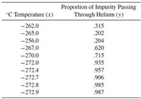
At temperatures approaching absolute zero (−273°C), helium exhibits traits that defy many laws of conventional physics. An experiment has been conducted with helium in solid form at various temperatures near absolute zero. The solid helium is placed in a dilution refrigerator along with a solid impure substance, and the fraction (in weight) of the impurity passing through the solid helium is recorded. (The phenomenon of solids passing directly through solids is known as quantum tunneling.) The data are given in the following table.

Chapter 11, Problem 95SE, At temperatures approaching absolute zero (273C), helium exhibits traits that defy many laws of

  1. a Fit a least-squares line to the data.
  2. b Test the null hypothesis H0 : β1 = 0 against the alternative hypothesis Ha : β1 < 0, at the α = .01 level of significance.
  3. c Find a 95% prediction interval for the percentage of the solid impurity passing through solid helium at −273◦C. (This value of x is outside the experimental region where use of the model for prediction may be dangerous.)

a.

Expert Solution
Check Mark
To determine

Fit a least-square line to the data.

Answer to Problem 95SE

The least-square line is y^=13.490350.05283x.

Explanation of Solution

The least-square line is as follows:

y^=β^0+β^1x

Where,

β^0=y¯β^1x¯, β1=SxySxx, Sxy=i=1n(xix¯)(yiy¯) and Sxx=i=1n(xix¯)2

x¯=1ni=1nxi, y¯=1ni=1nyi

From the table of data, the values of x¯ and y¯ can be computed as follows:

x¯=268.28, y¯=0.6826

Now, the values of Sxy and Sxx can be obtained as follows:

Sxy=i=110(xix¯)(yiy¯)=i=110(xi(268.28))(yi0.6826)=15.728

Thus, the value of Sxy is –15.728.

Sxx=i=1n(xix¯)2=i=1n(xi(268.28))2=297.716

The value of Sxx is 297.716.

Now, the values of slope and intercept are calculated as follows:

β^1=SxySxx=15.728297.716=0.05283

The value of slope β1 is –0.05283.

β^0=y¯β^1x¯=0.6826(0.05283)×(268.28)=13.49035

The value of intercept β^0 is –13.49035.

Substitute the value of intercept and slope in the model; then the model becomes,

y^=β^0+β^1xy^=13.490350.05283x

Thus, the least-square line is y^=13.490350.05283x.

b.

Expert Solution
Check Mark
To determine

Test the hypothesis H0:β1=0 against the alternative Ha:β1<0 at the 0.01 significance level.

Answer to Problem 95SE

There is sufficient evidence to conclude that β1 is less than zero.

Explanation of Solution

The null and alternative hypotheses are stated as follows:

H0:β1=0

Ha:β1<0

The significance level is 0.01.

The test statistic is as follows:

t=β^1(sc11)

Where,

β^1=SxySxx, Sxy=i=1n(xix¯)(yiy¯), and Sxx=i=1n(xix¯)2.

s=SSEn2, c11=1Sxx

SSE=Syyβ^1Sxy

From Part (a), it is seen that β^1=0.05283, Sxx=297.716, Sxy=15.728

Now, compute the value of Syy as follows:

Syy=i=1n(yiy¯)2=i=110(yi0.6826)2=0.97315

The value of Syy is 0.97315.

It is noticed that SSE=Syyβ^1Sxy.

SSE=Syyβ^1Sxy=0.97315(0.05283)(15.728)=0.14225

Thus, the value of SSE is 0.14225.

In addition, it is known that s=SSEn2, c11=1Sxx.

s=SSEn2=0.14225102=0.13335,

c11=1Sxx=1297.716=0.00336

The test statistic can be obtained as follows:

t=β^1(sc11)=0.05283(0.13335)0.003366.836

Thus, the test statistic value is –6.836.

Critical value:

Step-by-step procedure to obtain the t-critical value using Table 5 of Appendix 3:

  • Locate the degrees of freedom as 8 in the column of df.
  • Move left until column headed by t0.01.
  • Selecting the intersection of (8, 0.01) gives the critical value of t.

The critical value of t for the left-tailed test is 2.896.

Decision rule:

Reject the null hypothesis, if |tcal|>|ttab|, otherwise fail to reject the null hypothesis.

Conclusion:

The test statistic value is greater than the table value.

That is, (|tcal|=6.836)>(|ttab|=2.896).

Hence, by the rejection rule, reject the null hypothesis H0 at the 0.01 significance level.

Therefore, there is sufficient evidence to conclude that β1 is less than zero.

c.

Expert Solution
Check Mark
To determine

Find a 95% prediction interval for the percentage of the solid impurity passing through solid helium at 2730C.

Answer to Problem 95SE

A 95% prediction interval for the percentage of the solid impurity passing through solid helium is (0.599, 1.265).

Explanation of Solution

A 95% prediction interval for the percentage of the solid impurity passing through solid helium is as follows:

(β^0+β^1xt0.05.s1+1n+(xx¯)2Sxx, β^0+β^1x+t0.05.s1+1n+(xx¯)2Sxx )

From Part (a), it is obtained that,

β^0=13.49035, β^1=0.05283, Sxx=297.716, x¯=268.28, and n=10.

From Part (b), it is seen that the value of s=0.13335.

The t-critical value using Table 5 of Appendix 3 is t0.025=2.306.

The lower limit is computed as follows:

β^0+β^1xt0.025.s1+1n+(xx¯)2Sxx=13.490350.05283(273)2.306(0.13335)1+110+(273(268.28))2297.716=0.599

The upper limit is as follows:

 β^0+β^1x+t0.025.s1+1n+(xx¯)Sxx=13.490350.05283(273)+2.306(0.13335)1+110+(273(268.28))2297.716=1.265

Thus, a 95% prediction interval for the percentage of the solid impurity passing through solid helium is (0.599, 1.265).

Want to see more full solutions like this?

Subscribe now to access step-by-step solutions to millions of textbook problems written by subject matter experts!

Chapter 11 Solutions

MATH.STATISTICS W/APPL.>CUSTOM<

Ch. 11.3 - Some data obtained by C.E. Marcellari on the...Ch. 11.3 - Processors usually preserve cucumbers by...Ch. 11.3 - J. H. Matis and T. E. Wehrly report the following...Ch. 11.4 - a Derive the following identity:...Ch. 11.4 - An experiment was conducted to observe the effect...Ch. 11.4 - Prob. 17ECh. 11.4 - Prob. 18ECh. 11.4 - A study was conducted to determine the effects of...Ch. 11.4 - Suppose that Y1, Y2,,Yn are independent normal...Ch. 11.4 - Under the assumptions of Exercise 11.20, find...Ch. 11.4 - Prob. 22ECh. 11.5 - Use the properties of the least-squares estimators...Ch. 11.5 - Do the data in Exercise 11.19 present sufficient...Ch. 11.5 - Use the properties of the least-squares estimators...Ch. 11.5 - Let Y1, Y2, . . . , Yn be as given in Exercise...Ch. 11.5 - Prob. 30ECh. 11.5 - Using a chemical procedure called differential...Ch. 11.5 - Prob. 32ECh. 11.5 - Prob. 33ECh. 11.5 - Prob. 34ECh. 11.6 - For the simple linear regression model Y = 0 + 1x...Ch. 11.6 - Prob. 36ECh. 11.6 - Using the model fit to the data of Exercise 11.8,...Ch. 11.6 - Refer to Exercise 11.3. Find a 90% confidence...Ch. 11.6 - Refer to Exercise 11.16. Find a 95% confidence...Ch. 11.6 - Refer to Exercise 11.14. Find a 90% confidence...Ch. 11.6 - Prob. 41ECh. 11.7 - Suppose that the model Y=0+1+ is fit to the n data...Ch. 11.7 - Prob. 43ECh. 11.7 - Prob. 44ECh. 11.7 - Prob. 45ECh. 11.7 - Refer to Exercise 11.16. Find a 95% prediction...Ch. 11.7 - Refer to Exercise 11.14. Find a 95% prediction...Ch. 11.8 - The accompanying table gives the peak power load...Ch. 11.8 - Prob. 49ECh. 11.8 - Prob. 50ECh. 11.8 - Prob. 51ECh. 11.8 - Prob. 52ECh. 11.8 - Prob. 54ECh. 11.8 - Prob. 55ECh. 11.8 - Prob. 57ECh. 11.8 - Prob. 58ECh. 11.8 - Prob. 59ECh. 11.8 - Prob. 60ECh. 11.9 - Refer to Example 11.10. Find a 90% prediction...Ch. 11.9 - Prob. 62ECh. 11.9 - Prob. 63ECh. 11.9 - Prob. 64ECh. 11.9 - Prob. 65ECh. 11.10 - Refer to Exercise 11.3. Fit the model suggested...Ch. 11.10 - Prob. 67ECh. 11.10 - Fit the quadratic model Y=0+1x+2x2+ to the data...Ch. 11.10 - The manufacturer of Lexus automobiles has steadily...Ch. 11.10 - a Calculate SSE and S2 for Exercise 11.4. Use the...Ch. 11.12 - Consider the general linear model...Ch. 11.12 - Prob. 72ECh. 11.12 - Prob. 73ECh. 11.12 - An experiment was conducted to investigate the...Ch. 11.12 - Prob. 75ECh. 11.12 - The results that follow were obtained from an...Ch. 11.13 - Prob. 77ECh. 11.13 - Prob. 78ECh. 11.13 - Prob. 79ECh. 11.14 - Prob. 80ECh. 11.14 - Prob. 81ECh. 11.14 - Prob. 82ECh. 11.14 - Prob. 83ECh. 11.14 - Prob. 84ECh. 11.14 - Prob. 85ECh. 11.14 - Prob. 86ECh. 11.14 - Prob. 87ECh. 11.14 - Prob. 88ECh. 11.14 - Refer to the three models given in Exercise 11.88....Ch. 11.14 - Prob. 90ECh. 11.14 - Prob. 91ECh. 11.14 - Prob. 92ECh. 11.14 - Prob. 93ECh. 11.14 - Prob. 94ECh. 11 - At temperatures approaching absolute zero (273C),...Ch. 11 - A study was conducted to determine whether a...Ch. 11 - Prob. 97SECh. 11 - Prob. 98SECh. 11 - Prob. 99SECh. 11 - Prob. 100SECh. 11 - Prob. 102SECh. 11 - Prob. 103SECh. 11 - An experiment was conducted to determine the...Ch. 11 - Prob. 105SECh. 11 - Prob. 106SECh. 11 - Prob. 107SE
Knowledge Booster
Background pattern image
Statistics
Learn more about
Need a deep-dive on the concept behind this application? Look no further. Learn more about this topic, statistics and related others by exploring similar questions and additional content below.
Recommended textbooks for you
Text book image
MATLAB: An Introduction with Applications
Statistics
ISBN:9781119256830
Author:Amos Gilat
Publisher:John Wiley & Sons Inc
Text book image
Probability and Statistics for Engineering and th...
Statistics
ISBN:9781305251809
Author:Jay L. Devore
Publisher:Cengage Learning
Text book image
Statistics for The Behavioral Sciences (MindTap C...
Statistics
ISBN:9781305504912
Author:Frederick J Gravetter, Larry B. Wallnau
Publisher:Cengage Learning
Text book image
Elementary Statistics: Picturing the World (7th E...
Statistics
ISBN:9780134683416
Author:Ron Larson, Betsy Farber
Publisher:PEARSON
Text book image
The Basic Practice of Statistics
Statistics
ISBN:9781319042578
Author:David S. Moore, William I. Notz, Michael A. Fligner
Publisher:W. H. Freeman
Text book image
Introduction to the Practice of Statistics
Statistics
ISBN:9781319013387
Author:David S. Moore, George P. McCabe, Bruce A. Craig
Publisher:W. H. Freeman
01 - What Is A Differential Equation in Calculus? Learn to Solve Ordinary Differential Equations.; Author: Math and Science;https://www.youtube.com/watch?v=K80YEHQpx9g;License: Standard YouTube License, CC-BY
Higher Order Differential Equation with constant coefficient (GATE) (Part 1) l GATE 2018; Author: GATE Lectures by Dishank;https://www.youtube.com/watch?v=ODxP7BbqAjA;License: Standard YouTube License, CC-BY
Solution of Differential Equations and Initial Value Problems; Author: Jefril Amboy;https://www.youtube.com/watch?v=Q68sk7XS-dc;License: Standard YouTube License, CC-BY