Videos
In Exercises 5–20, conduct the hypothesis test and provide the test statistic and the P-value and /or critical value, and state the conclusion.
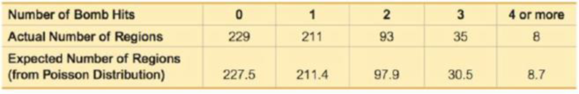
10. Do World War II Bomb Hits Fit a Poisson Distribution? In analyzing hits by V-l buzz bombs in World War II, South London was subdivided into regions, each with an area of 0.25 km2. Shown below is a table of actual frequencies of hits and the frequencies expected with the Poisson distribution. (The Poisson distribution is described in Section 5-3.) Use the values listed and a 0.05 significance level to test the claim that the actual frequencies fit a Poisson distribution. Does the result prove that the data conform to the Poisson distribution?
Want to see the full answer?
Check out a sample textbook solution
Chapter 11 Solutions
MyLab Statistics with Pearson eText -- Standalone Access Card -- for Elementary Statistics


- What is meant by the sample space of an experiment?arrow_forwardIn Exercises 5–16, use the listed paired sample data, and assume that the samples are simple random samples and that the differences have a distribution that is approximately normal. Heights of Fathers and Sons Listed below are heights (in.) of fathers and their first sons. The data are from a journal kept by Francis Galton. (See Data Set 5 “Family Heights” in Appendix B.) Use a 0.05 significance level to test the claim that there is no difference in heights between fathers and their first sons.arrow_forwardIn Exercises 5–16, use the listed paired sample data, and assume that the samples are simple random samples and that the differences have a distribution that is approximately normal. Heights of Mothers and Daughters Listed below are heights (in.) of mothers and their first daughters. The data are from a journal kept by Francis Galton. (See Data Set 5 “Family Heights” in Appendix B.) Use a 0.05 significance level to test the claim that there is no difference in heights between mothers and their first daughters.arrow_forward
- 4. Define what is a Sampling Distribution of Sample Means and how it correlates to the Central Limit Theorem? 5. Define what is a Confidence Interval in Statistics and how we can apply it to a real life situation?arrow_forwardIn Exercises 5–16, use the listed paired sample data, and assume that the samples are simple random samples and that the differences have a distribution that is approximately normal. Heights of Presidents A popular theory is that presidential candidates have an advantage if they are taller than their main opponents. Listed are heights (cm) of presidents along with the heights of their main opponents (from Data Set 15 “Presidents”). a. Use the sample data with a 0.05 significance level to test the claim that for the population of heights of presidents and their main opponents, the differences have a mean greater than 0 cm. b. Construct the confidence interval that could be used for the hypothesis test described in part (a). What feature of the confidence interval leads to the same conclusion reached in part (a)?arrow_forwardIn Exercises 5–16, use the listed paired sample data, and assume that the samples are simple random samples and that the differences have a distribution that is approximately normal. Speed Dating: Attractiveness Listed below are “attractiveness” ratings made by participants in a speed dating session. Each attribute rating is the sum of the ratings of five attributes (sincerity, intelligence, fun, ambition, shared interests). The listed ratings are from Data Set 18 “Speed Dating.” Use a 0.05 significance level to test the claim that there is a difference between female attractiveness ratings and male attractiveness ratings.arrow_forward
- In Exercises 5–16, use the listed paired sample data, and assume that the samples are simple random samples and that the differences have a distribution that is approximately normal. Speed Dating: Attributes Listed below are “attribute” ratings made by participants in a speed dating session. Each attribute rating is the sum of the ratings of five attributes (sincerity, intelligence, fun, ambition, shared interests). The listed ratings are from Data Set 18 “Speed Dating” in Appendix B. Use a 0.05 significance level to test the claim that there is a difference between female attribute ratings and male attribute ratings.arrow_forwardIn Exercises 5–16, use the listed paired sample data, and assume that the samples are simple random samples and that the differences have a distribution that is approximately normal. Two Heads Are Better Than One Listed below are brain volumes (cm3 ) of twins from Data Set 8 “IQ and Brain Size” in Appendix B. Construct a 99% confidence interval estimate of the mean of the differences between brain volumes for the first-born and the second-born twins. What does the confidence interval suggest?arrow_forwardAs part of a quality control process for computer chips, an engineer at a factory randomly samples 212 chips during a week of production to test the current rate of chips with severe defects. She finds that 50 of the chips are defective. A. What is the population under consideration in the data set? B.What parameter is being estimated? C. What is the point estimate for the parameter? D. The historical rate of defects at the factory is 10%. If this is still the rate of defects, describe the sampling distribution of sample proportions of defective chips. Be sure to check the appropriate conditions and include the shape, center, spread, and a well-labeled sketch of the sampling distribution. E. Based on your sketch from Part (D) and the point estimate you found in Part (C), do you think the rate of defects is still 10%? Why or why not?arrow_forward
- The National Center for Education Statistics reports that the proportion of college freshmen who return to the same school for their sophomore year is 0.71. Suppose we select a random sample of 490 freshmen from across the nation. What is the expected value of the sampling distribution model for the proportion of 490 freshmen that will return to the same school for their sophomore year? a) What is the standard deviation of the sampling distribution model for the proportion of 490 freshmen that will return to the same school for their sophomore year? b) What is the probability that the proportion of these 490 freshmen that return to the same school for their sophomore year is less than 0.66?arrow_forward1a. If the parameter is 5.5, which sampling distribution are unbiased? Why? 1b. Which of the sampling distributions is the best estimator of the parameter? Why? 1c. Which of the choices has low variability and high bias? Why?arrow_forward
 Holt Mcdougal Larson Pre-algebra: Student Edition...AlgebraISBN:9780547587776Author:HOLT MCDOUGALPublisher:HOLT MCDOUGAL
 College Algebra (MindTap Course List)AlgebraISBN:9781305652231Author:R. David Gustafson, Jeff HughesPublisher:Cengage Learning