
Videos
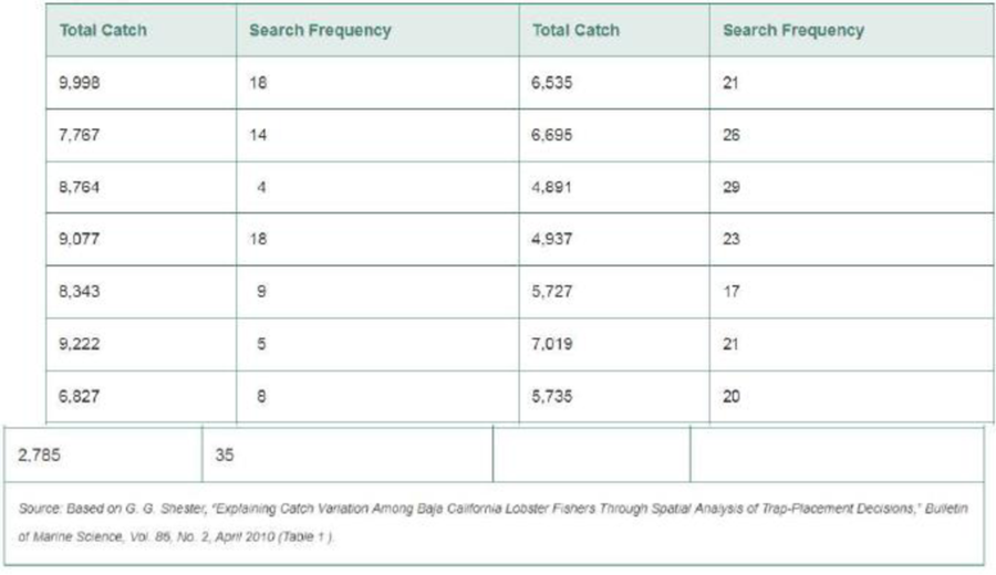
Lobster fishing study. Refer to the Bulletin of Marine Science (April 2010) study of teams of fishermen fishing for the red spiny lobster in Baja California Sur, Mexico, Exercise 2.126 (p. 107). Two variables measured for each of 15 teams from two fishing cooperatives were y = total catch of lobsters (in kilograms) during the season and x = average percentage of traps allocated per day to exploring areas of unknown catch (called search frequency). These data are listed in the table.
a. Graph the data in a
b. A simple linear
c. If possible, give a practical interpretation of the estimate of β0. If no practical interpretation is possible, explain why.
d. If possible, give a practical interpretation of the estimate of β1. If no practical interpretation is possible, explain why.
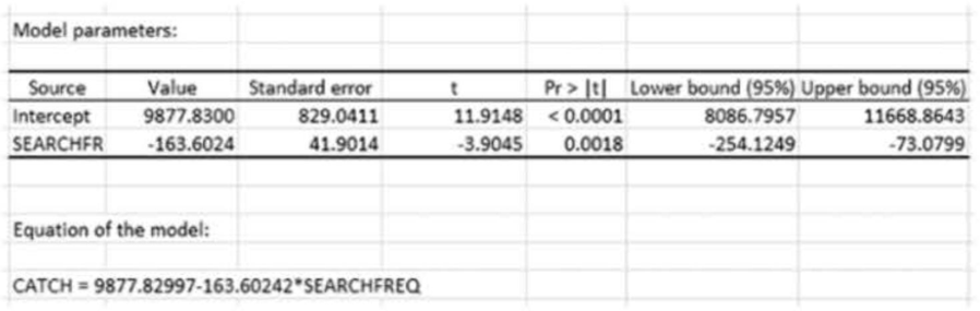
XLSTAT output for Exercise 11.2
Want to see the full answer?
Check out a sample textbook solution
Chapter 11 Solutions
Statistics for Business and Economics, Student Value Edition (13th Edition)


- Urban Travel Times Population of cities and driving times are related, as shown in the accompanying table, which shows the 1960 population N, in thousands, for several cities, together with the average time T, in minutes, sent by residents driving to work. City Population N Driving time T Los Angeles 6489 16.8 Pittsburgh 1804 12.6 Washington 1808 14.3 Hutchinson 38 6.1 Nashville 347 10.8 Tallahassee 48 7.3 An analysis of these data, along with data from 17 other cities in the United States and Canada, led to a power model of average driving time as a function of population. a Construct a power model of driving time in minutes as a function of population measured in thousands b Is average driving time in Pittsburgh more or less than would be expected from its population? c If you wish to move to a smaller city to reduce your average driving time to work by 25, how much smaller should the city be?arrow_forwardA research group is interested in the relationship between exposure to mold in households after a major hurricane and the onset of acute respiratory illness in children. Suppose an observational study is conducted over 10 years following the natural disaster and the following two-by-two table was created in order to address the relationship between exposure and outcome. Acute Respiratory Illness No Acute Respiratory Illness Total Mold 378 156 534 No Mold 73 260 333 Total 451 416 867 Calculate the incidence of acute respiratory illness in the exposed and unexposed. Calculate the relative risk for ARI due to exposure in this study Interpret your findings from part Barrow_forwardIn a study on television violence and aggression, researchers measured the TV viewing habits of 3rd grade males (preference for violent TV shows) and their levels of aggression; and then revisited the men 10 years later and measured the same variables. They found these zero-order correlations: Aggression G3 TV G3 Aggression Y18 Aggression G3 1.0 .65 .45 TV G3 1.0 .5 Aggression Y18 1.0 a) Suggest an operational definition to measure TV show preference for violent TV shows at Grade 3 and at Year 18. b) What is going on if the partial correlation of TV G3 and AGG Y18 with AGG G3 held constant is .09? How do you know this? c) What is going on if the partial correlation of AGG G3 and AGG Y18 with TV G3 held constant is .06? How do you know this?arrow_forward
- The Turbine Oil Oxidation Test (TOST) and the Rotating Bomb Oxidation Test (RBOT) are two different procedures for evaluating the oxidation stability of steam turbine oils. An article reported the accompanying observations for x = TOST time (hr) and y = RBOT time (min) for 12 oil specimens. TOST 4200 3575 3750 3700 4050 2770 4870 4475 3450 2700 3750 3325 RBOT 370 345 375 310 350 205 400 375 285 220 345 280 (a) Calculate the value of the sample correlation coefficient. (Round your answer to four decimal places.)r = Interpret the value of the sample correlation coefficient. The value of r indicates that there is a strong, negative linear relationship between TOST and RBOT.The value of r indicates that there is a weak, positive linear relationship between TOST and RBOT. The value of r indicates that there is a strong, positive linear relationship between TOST and RBOT.The value of r indicates that there is a weak, negative…arrow_forwardDetermine the critical values of r and if it represents a significant linear correlation.arrow_forwardA survey of high school students was done to examine whether students had ever driven a car after consuming a substantial amount of alcohol (1=yes, 0=no). Data was collected on their sex (male/female), race (White/non-White), and grade level (9,10,11,12). Researchers realized that the impact of race on consuming alcohol before driving might vary by grade level and decided to fit the following model. Variable Coding = 1 if Intercept Sex () Female Race () Black Grade level ( 9th grade 10th grade 11th grade [Reference = 12th grade] Attached is the logistic model 1. Compute the OR of drinking before driving for students who self-reported as Black versus non-Black in the 9th grade, adjusting for gender. 2. Compute the OR of drinking before driving for students who self-reported as Black versus non-Black in the 12th grade, adjusting for gender. 3. Compute the OR of drinking before driving for someone in the 9th grade versus 12th grade for a student who…arrow_forward
 Functions and Change: A Modeling Approach to Coll...AlgebraISBN:9781337111348Author:Bruce Crauder, Benny Evans, Alan NoellPublisher:Cengage Learning
 Glencoe Algebra 1, Student Edition, 9780079039897...AlgebraISBN:9780079039897Author:CarterPublisher:McGraw Hill
 Big Ideas Math A Bridge To Success Algebra 1: Stu...AlgebraISBN:9781680331141Author:HOUGHTON MIFFLIN HARCOURTPublisher:Houghton Mifflin Harcourt