
Concept explainers
Videos
The paper “Less Air Pollution Leads to Rapid Reduction of Airway Inflammation and Improved Airway
The authors of the paper used paired t tests to determine that there was a significant difference in the urban and rural means for each of these three measures. One of these tests resulted in a P-value less than 0.001, one resulted in a P-value between 0.001 and 0.01, and one resulted in a P-value between 0.01 and 0.05.
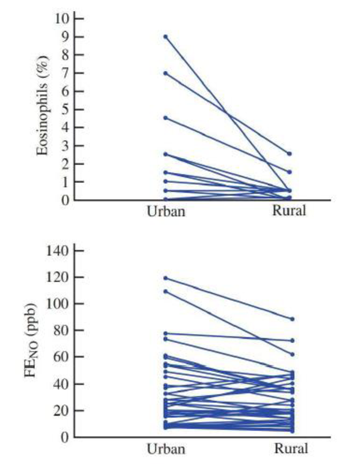
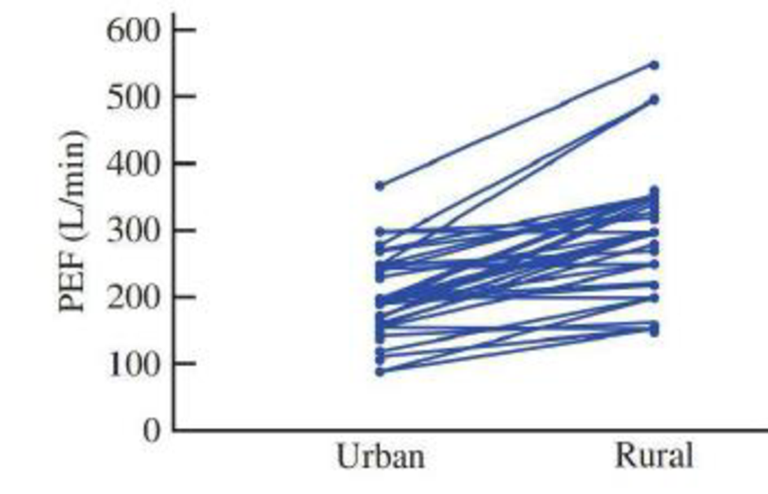
- a. Which measure (Eosinophils, FENO, or PEF) do you think resulted in a test with the P-value that was less than 0.001? Explain your reasoning.
- b. Which measure (Eosinophils, FENO, or PEF) do you think resulted in the test with the largest P-value? Explain your reasoning.
Want to see the full answer?
Check out a sample textbook solution
Chapter 11 Solutions
Bundle: Introduction to Statistics and Data Analysis, 5th + WebAssign Printed Access Card: Peck/Olsen/Devore. 5th Edition, Single-Term


- Reduced heart rate variability (HRV) is known to be a predictor of mortality after a heart attack. One measure of HRV is the average normal-to-normal beat interval (in milliseconds) for a 24-hr time period. Twenty-two heart attack patients who were dog owners and 80 heart attack patients who did not own a dog participated in a study of the effect of pet ownership on HRV, resulting in the summary statistics shown in the accompanying table. Measure of HRV(Average Normal-to-Normal Beat Interval) Mean StandardDeviation Owns Dog 871 134 Does Not Own Dog 800 138 (b) The paper indicates that the null hypothesis in part (a) was rejected and reported that the P-value was less than 0.05. Carry out a two-sample t test. (Use ? = 0.05. Use ?1 for heart attack patients who are dog owners and ?2 for heart attack patients who do not own a dog.) Find the test statistic and P-value. (Use SALT. Round your test statistic to one decimal place and your P-value to three decimal places.) t=…arrow_forwardReduced heart rate variability (HRV) is known to be a predictor of mortality after a heart attack. One measure of HRV is the average of normal-to-normal beat interval (in milliseconds) for a 24-hour time period. Twenty-two heart attack patients who were dog owners and 80 heart attack patients who did not own a dog participated in a study of the effect of pet ownership on HRV, resulting in the summary statistics shown in the accompanying table. Measure ofHRV (averagenormal-to-normalbeat interval) Mean StandardDeviation Owns Dog 874 136 Does Not Own Dog 801 133 (a) The authors of this paper used a two-sample t test to test H0: ?1 - ?2 = 0 versus Ha: ?1 - ?2 ≠ 0. What assumptions must be reasonable in order for this to be an appropriate method of analysis?We must assume that the population distributions ---Select--- are aren't approximately normal.(b) The paper indicates that the null hypothesis from Part (a) was rejected and reports that the P-value is less than…arrow_forwardA cohort study is conducted to assess the association between clinical characteristics and the risk of stroke. The study involves n=1,250 participants who are free of stroke at the study start. Each participant is assessed at study start (baseline) and every year thereafter for five years. The following table displays data on hypertensive status measured at baseline and incident stroke over 5 years. Free of Stroke at 5 Years Stroke Baseline: Not Hypertensive 952 46 Baseline: Hypertensive 234 18 Compute the population attributable risk of stroke for patients with hypertension.arrow_forward
- A cohort study is conducted to assess the association between clinical characteristics and the risk of stroke. The study involves n=1,250 participants who are free of stroke at the study start. Each participant is assessed at study start (baseline) and every year thereafter for five years. The following table displays data on hypertensive status measured at baseline and incident stroke over 5 years. Free of Stroke at 5 Years Stroke Baseline: Not Hypertensive 952 46 Baseline: Hypertensive 234 18 Compute the risk difference of stroke (per 5 person-years) for patients with hypertension as compared to patients free of hypertension.arrow_forwardA cohort study is conducted to assess the association between clinical characteristics and the risk of stroke. The study involves n=1,250 participants who are free of stroke at the study start. Each participant is assessed at study start (baseline) and every year thereafter for five years. The following table displays data on hypertensive status measured at baseline and incident stroke over 5 years. Free of Stroke over 5 Years Stroke Baseline: Not Hypertensive 952 46 Baseline: Hypertensive 234 18 Compute the cumulative incidence of stroke in the study.arrow_forwardEstriol Level and Birth Weight. J. Greene and J. Touchstone conducted a study on the relationship between the estriol levels of pregnant women and the birth weights of their children. Their findings, “Urinary Tract Estriol: An Index of Placental Function,” were published in the American Journal of Obstetrics and Gynecology (Vol. 85(1), pp. 1–9). The data from the study are provided on the WeissStats site, where estriol levels are in mg/24 hr and birth weights are in hectograms. a. Decide whether finding a regression line for the data is reasonable. If so, then also do parts (b)–(d). b. Obtain the coefficient of determination. c. Determine the percentage of variation in the observed values of the response variable explained by the regression, and interpret your answer. d. State how useful the regression equation appears to be for making predictions.arrow_forward
- Efforts by airlines to improve on-time arrival rates are showing results. Boston.com reports that in the first 10 months of 2012 on-time arrival rates at U.S. airports were the highest they have been since 2003. During this period 82% of flights landed within 15 minutes of their scheduled time. Are there differences among the major airlines? The data in Sheet 35 show the number of on-time arrivals for samples of flight taken from seven major U.S. airlines in 2012. Using a 0.05 level of significance, what is the p-value and what is your conclusion? Sheet 35 Arrivals American Airlines Continental Airlines Delta Airlines JetBlue Airlines Southwest Airlines United Airlines US Airways On-time 83 54 96 60 69 66 68 Late 16 18 21 22 23 15 12 99 72 117 82 92 81 80 Select one: a) Chi-square statistic = 4.32, p-value = 0.034, reject the null hypothesis, there is a statistically significant differences in the proportion of on-time arrivals b) Chi-square statistic = 7.370,…arrow_forwardRetinitis pigmentosa (RP) is a hereditary ocular diseasein which patches of pigment appear on the retina, potentially resulting in substantial vision loss and in somecases complete blindness. An important issue is how fastthe subjects decline. Visual field is an important measureof area of vision, which is measured in degree2. A visualfield area for a normal person is around 11,000 degree2.The longitudinal data in Table 11.29 were provided by anindividual patient.Table 11.29 Longitudinal visual field data forone RP patientTime Visual field area lnVisit (yr) (degree2) (visual field area)1 0 3059 8.032 1 3053 8.023 2 1418 7.264 3 1692 7.435 4 1978 7.596 5 1567 7.367 6 1919 7.568 7 1998 7.609 11 1648 7.4110 13 1721 7.4511 15 1264 7.14mean 6.09 1938 7.532sd 4.97 597 0.280Suppose the rate of change of ln (visual field) is a linearfunction of follow-up time.11.103 Write down a linear regression model that summarizes this relationship.11.104 Fit the regression line using the method of…arrow_forwardAn article in Plant Disease, "Effect of Nitrogen and Potassium Fertilizer Rates on Severity of Xanthomonas Blight of Syngonium Podophyllum" (1989, Vol. 73, No. 12, pp. 972-975) showed the effect of the variable nitrogen and potassium rates on the growth of "White Butterfly" and the mean percentage of disease. Data representative of that collected in this experiment is provided in the following table. Potassium (mg/pot/wk) Nitrogen (mg/pot/wk) 30 90 120 50 60.8 60.8 45.5 43.0 60.0 58.4 150 54.4 56.1 53.8 51.6 34.5 35.5 250 42.9 40.0 36.1 37.9 33.0 33.3 (a) Use the analysis of variance to test the appropriate hypotheses with a = 0.05. The effect of the variable nitrogen significant, the effect of the potassium rates significant, the interaction between the variable nitrogen and potassium rates significant. (b) Graphically analyze the residuals from this experiment. The residuals acceptable. (c) Estimate the appropriate variance component. Round your answers to 2 decimal places. Source…arrow_forward
- The income of males in each state of the United States, including the District of Columbia and Puerto Rico, are given in table #9.3.3, and the income of females is given in table #9.3.4 ("Median income of," 2013). Is there enough evidence to show that the mean income of males is more than of females? Test at the 1% level. (Show the work) Table #9.3.3: Data of Income for Males $42,951 $52,379 $42,544 $37,488 $49,281 $50,987 $60,705 $50,411 $66,760 $40,951 $43,902 $45,494 $41,528 $50,746 $45,183 $43,624 $43,993 $41,612 $46,313 $43,944 $56,708 $60,264 $50,053 $50,580 $40,202 $43,146 $41,635 $42,182 $41,803 $53,033 $60,568 $41,037 $50,388 $41,950 $44,660 $46,176 $41,420 $45,976 $47,956 $22,529 $48,842 $41,464 $40,285 $41,309 $43,160 $47,573 $44,057 $52,805 $53,046 $42,125 $46,214 $51,630 Table #9.3.4: Data of Income for Females $31,862…arrow_forwardForest bathing, also called Shinrin-yoke, is the practice of taking short, leisurely walks in a forest to enhance positive health. To test if forest bathing and mood are related, a clinical psychologist records the time spent forest bathing in minutes (X) and the corresponding change I mood using a standard self report affect grid (Y) among 8 patients with a history of depression. The data are given in the following table. times spent forest bathing (in minutes) change in mood X Y 32 +24 24 +20 28 +25 17 +22 12 +16 Compute the method of least squares to find the equation of the regression line. Use the regression equation computed in part (a) to determine the predicted change in mood of a person who spends 20 minutes forest bathing.arrow_forwardThe size of the left upper chamber of the heart is one measure of cardiovascular health. When the upper left chamber is enlarged, the risk of heart problems is increased. The paper “Left Atrial Size Increases with Body Mass Index in Children” (International Journal of Cardiology [2009]:1-7) described a study in which the left atrial size was measured for a large number of children age 5 to 15 years. Based on this data, the authors concluded that for healthy children, left atrial diameter was approximately normally distributed with a mean of 26.4 mm and a standard deviation of 4.2 mm. Approximately what proportion of healthy children has left atrial diameters less than 24 mm? Approximately what proportion of healthy children has left atrial diameters greater than 32 mm? Approximately what proportion of healthy children has left atrial diameters between 25 and 30 mm? For healthy children, what is the value for which only about 20% have a larger left atrial diameter?arrow_forward
 Linear Algebra: A Modern IntroductionAlgebraISBN:9781285463247Author:David PoolePublisher:Cengage Learning
 Glencoe Algebra 1, Student Edition, 9780079039897...AlgebraISBN:9780079039897Author:CarterPublisher:McGraw Hill
 Big Ideas Math A Bridge To Success Algebra 1: Stu...AlgebraISBN:9781680331141Author:HOUGHTON MIFFLIN HARCOURTPublisher:Houghton Mifflin Harcourt