
Concept explainers
Videos
If the null hypothesis is rejected in Exercises 1 through 8, use the Scheffé test when the sample sizes are unequal to test the differences between the means, and use the Tukey test when the sample sizes are equal. For these exercises, perform these steps. Assume the assumptions have been met.
a. State the hypotheses and identify the claim.
b. Find the critical value(s).
c. Compute the test value.
d. Make the decision.
e. Summarize the results.
Use the traditional method of hypothesis testing unless otherwise specified.
1. Lengths of Various Types of Bridges The data represent the lengths in feet of three types of bridges in the United States. At a = 0.01, test the claim that there is no significant difference in the means of the lengths of the types of bridges.
| Simple truss | Segmented concrete | Continuous plate |
| 745 | 820 | 630 |
| 716 | 750 | 573 |
| 700 | 790 | 525 |
| 650 | 674 | 510 |
| 647 | 660 | 480 |
| 625 | 640 | 460 |
| 608 | 636 | 451 |
| 598 | 620 | 450 |
| 550 | 520 | 450 |
| 545 | 450 | 425 |
| 534 | 392 | 420 |
| 528 | 370 | 360 |
a.
To state: The hypothesis
To identify: The claim.
Answer to Problem 12.1.1RE
The hypothesis
The claim is that, all the means are same.
Explanation of Solution
Given info:
The data shows the lengths in feet of three types of bridges in the United States. The level of significance is 0.01.
Calculation:
The hypotheses are given below:
Null hypothesis:
Alternative hypothesis:
Here, all the means are same is tested. Hence, the claim is that, all the means are same.
b.
To find: The critical value.
Answer to Problem 12.1.1RE
The critical value is 5.285.
Explanation of Solution
Given info:
The level of significance is 0.01. The number of samples k is 3, the sample sizes
Calculation:
The degrees of freedom are
Where
Substitute 3 for k in
Substitute 36 for N and 3 for k in
Critical value:
The critical F-value is obtained using the Table H: The F-Distribution with the level of significance
Procedure:
- Locate 30 and 40 in the degrees of freedom, denominator row of the Table H.
- Obtain the value in the corresponding degrees of freedom, numerator column below 2.
That is,
That is, the critical value is 5.285.
Rejection region:
The null hypothesis would be rejected if
c.
To compute: The test value.
Answer to Problem 12.1.1RE
The test value is 6.94.
Explanation of Solution
Calculation:
Software procedure:
Step-by-step procedure to obtain the test statistic using the MINITAB software:
- Choose Stat > ANOVA > One-Way.
- In Response, enter the Temperatures.
- In Factor, enter the Factor.
- Click OK.
Output using the MINITAB software is given below:
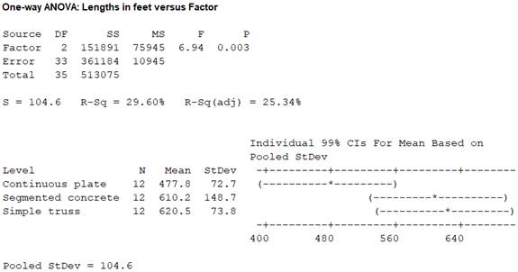
From the MINITAB output, the test value F is 6.94.
d.
To make: The decision.
Answer to Problem 12.1.1RE
The null hypothesis is rejected.
Explanation of Solution
Conclusion:
From the result of part (c), the test value is 6.94.
Here, the F-statistic value is greater than the critical value.
That is,
Thus, it can be concluding that, the null hypothesis is rejected.
e.
To explain: The results.
Answer to Problem 12.1.1RE
The result concludes that, there is a significant difference between the means
Explanation of Solution
Calculation:
From the results, it can be observed that the null hypothesis is rejected. Thus, it can be concluding that there is evidence to reject the claim that all means are same.
Consider,
Step-by-step procedure to obtain the test mean and standard deviation using the MINITAB software:
- Choose Stat > Basic Statistics > Display Descriptive Statistics.
- In Variables enter the columns Florida, Pennsylvania and Maine.
- Choose option statistics, and select Mean, Variance and N total.
- Click OK.
Output using the MINITAB software is given below:
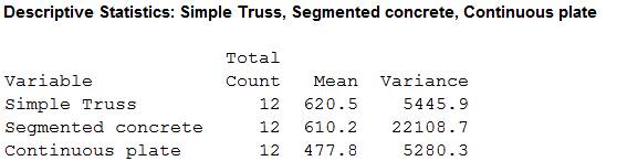
The sample sizes
The means are
The sample variances are
Here, the samples of sizes of three states are equal. So, the test used here is Tukey test.
Tukey test:
Critical value:
Here, k is 3 and degrees of freedom
Substitute 36 for N and 3 for k in v
The critical F-value is obtained using the Table N: Critical Values for the Tukey test with the level of significance
Procedure:
- Locate nearest value of 33 in the column of v of the Table H.
- Obtain the value in the corresponding row below 3.
That is, the critical value is 4.45.
Comparison of the means:
The formula for finding
That is,
Comparison between the means
The hypotheses are given below:
Null hypothesis:
Alternative hypothesis:
Rejection region:
The null hypothesis would be rejected if absolute value greater than the critical value.
Absolute value:
The formula for comparing the means
Substitute 620.5 and 610.2 for
Thus, the value of
Hence, the absolute value of
Conclusion:
The absolute value is 0.34.
Here, the absolute value is lesser than the critical value.
That is,
Thus, the null hypothesis is not rejected.
Hence, there is no significant difference between the means
Comparison between the means
The hypotheses are given below:
Null hypothesis:
Alternative hypothesis:
Rejection region:
The null hypothesis would be rejected if absolute value greater than the critical value.
Absolute value:
The formula for comparing the means
Substitute 620.5 and 477.8 for
Thus, the value of
Hence, the absolute value of
Conclusion:
The absolute value is 4.72.
Here, the absolute value is greater than the critical value.
That is,
Thus, the null hypothesis is rejected.
Hence, there is significant difference between the means
Comparison between the means
The hypotheses are given below:
Null hypothesis:
Alternative hypothesis:
Rejection region:
The null hypothesis would be rejected if absolute value greater than the critical value.
Absolute value:
The formula for comparing the means
Substitute 610.2 and 477.8 for
Thus, the value of
Hence, the absolute value of
Conclusion:
The absolute value is 4.38.
Here, the absolute value is lesser than the critical value.
That is,
Thus, the null hypothesis is not rejected.
Hence, there is no significant difference between the means
Want to see more full solutions like this?
Chapter 12 Solutions
ELEMENTARY STATISTICS: STEP BY STEP- ALE


- In each of Exercises, we have provided a null hypothesis and alternative hypothesis and a sample from the population under consideration. In each case, use theWilcoxon signed-rank test to perform the required hypothesis test at the 10% significance level. H0: µ = 10, Ha: µ<10 7 6 5 12 15 14 13 4arrow_forwardAfter running a hypothesis test comparing the number of jelly beans that a sample of children eat over the course of the year with the number of jelly beans children eat in the overall population over the course of the year, I conclude that the sample of children ate significantly more jelly beans than the overall population of children. If the sample of children actually ate the same number of jelly beans as the overall population, my conclusion is an example of _______. a. sampling error b. a Type II error c. a Type I error d. a valid conclusionarrow_forwardA company that produces snack foods uses a machine to package 454g bags of pretzels. The hypotheses are as follows: Ho : µ = 454g (the packaging machine is working properly) Ha : µ ≠ 454g (the packaging machine is not working properly) Suppose that the results of the sampling lead to accepting of the null hypothesis. Classify the conclusion as a Type I Error, Type II Error, or a correct decision, if in fact the mean net weight is not equal to 454g.arrow_forward
- A fast-food restaurant claims that a small order of french fries contains 120 calories. A nutritionist is concerned that the true average calorie count is higher than that. The nutritionist randomly selects 35 small orders of french fries and determines their calories. The resulting sample mean is 155.6 calories, and the pp-value for the hypothesis test is 0.00093. Which of the following is a correct interpretation of the p-value? A)If the population mean is 120 calories, the p -value of 0.00093 is the probability of observing a sample mean of 155.6 calories or more. B) If the population mean is 120 calories, the p -value of 0.00093 is the probability of observing a sample mean of 155.6 calories or less. C)If the population mean is 120 calories, the p -value of 0.00093 is the probability of observing a sample mean of 155.6 calories or more, or a sample mean of 84.4 calories or less. .D)If the population mean is 155.6 calories, the p -value of 0.00093…arrow_forwardGiven the sample data below, test the claim thatthe proportion of male voters who plan to vote Republican at the nextpresidential election is greater than the percentage of female voters who plan to vote Republican. State the Null and Alternative hypotheses.Use the P-value method of hypothesis testing and use a significance level of 0.10. Men: n1= 250, x1= 146 Women: n2= 202, x2= 103arrow_forwardFor a one-sample test for a population proportion pp and sample size nn, why is it necessary that np0np0 and n(1−p0)n(1−p0) are both at least 10 ? A)The sample size must be large enough to support an assumption that the distribution of the population is approximately normal. B)The sample size must be large enough to support an assumption that the distribution of the sample is approximately normal. C)The sample size must be large enough to support an assumption that the sampling distribution of the sample proportion is approximately normal. D)The sample size must be large enough to support an assumption that the observations are independent. E)The sample size must be large enough to support an assumption that the sample proportion is an unbiased estimator of the population proportion.arrow_forward
- Are the requirements met to test a hypothesis for the following two population proportions? If not, state which requirement is not met, and show whyit fails. In a random sample of 100car owners, 85% said they were happy with the fuel economy of their car. In a random sample of 80truck owners, 4% said they were happy with the fuel economy of their truck.arrow_forwardGiven the two independent samples below, conduct a hypothesis test for the desired scenario. Assume all populations are approximately normally distributed. Sample 1 Sample 2 n1= 971 n2=n2= 707 ¯x1=375 ¯x2=448 s1=150 s2= 179 Test the claim: Given the null and alternative hypotheses below, conduct a hypothesis test for α=0.01α=0.01.H0H0: μ1=μ2HaHa: μ1>μ2 Given the alternative hypothesis, the test is Determine the test statistic. Round to four decimal places.t=t= Find the pp-value. Round to 4 decimals.pp-value = Make a decision. Fail to reject the null hypothesis. Reject the null hypothesis.arrow_forwardUsing the data in the Excel file consumer Transportation Survey, test the following null hypotheses: Individuals drive an average of 600 miles per week. Vehicle Driven Miles driven per week Truck 450 Truck 370 Truck 580 Truck 300 SUV 1000 SUV 840 SUV 1400 SUV 300 SUV 850 SUV 700 SUV 350 SUV 1500 SUV 280 SUV 400 SUV 420 SUV 675 SUV 800 SUV 300 SUV 400 Mini Van 400 Mini Van 700 Mini Van 720 Mini Van 450 Mini Van 1000 Mini Van 350 Mini Van 800 Mini Van 200 Mini Van 350 Car 150 Car 175 Car 355 Car 150 Car 600 Car 600 Car 300 Car 275 Car 285 Car 400 Car 350 Car 600 Car 700 Car 600 Car 400 Car 350 Car 250 Car 355 Car 175 Car 300 Car 350 Car 500arrow_forward
- AND THE P VALUE FOR THE TEST HYPOTHESISarrow_forwardGiven the following null and alternative hypotheses H0: µ1 - µ2 = 0 HA: µ1 - µ2 ≠ 0 and the following sample information Sample 1 Sample 2 n1 = 125 n2 = 120 s1 = 31 s2 = 38 x1 = 130 x2 = 105 Develop the appropriate decision rule, assuming a significance level of 0.05 is to be used. Test the null hypothesis and indicate whether the sample information leads you to reject or fail to reject the null hypothesis. Use the test statistic approach.arrow_forwardIf all other factors are held constant, which of the following results in a decrease in the probability of a Type IIII error? The true parameter is closer to the value of the null hypothesis. A The sample size is decreased. B The significance level is decreased. C The standard error is decreased. D The probability of a Type IIII error cannot be decreased, only increased. Earrow_forward
 MATLAB: An Introduction with ApplicationsStatisticsISBN:9781119256830Author:Amos GilatPublisher:John Wiley & Sons Inc
 Probability and Statistics for Engineering and th...StatisticsISBN:9781305251809Author:Jay L. DevorePublisher:Cengage Learning
 Statistics for The Behavioral Sciences (MindTap C...StatisticsISBN:9781305504912Author:Frederick J Gravetter, Larry B. WallnauPublisher:Cengage Learning
 Elementary Statistics: Picturing the World (7th E...StatisticsISBN:9780134683416Author:Ron Larson, Betsy FarberPublisher:PEARSON
 The Basic Practice of StatisticsStatisticsISBN:9781319042578Author:David S. Moore, William I. Notz, Michael A. FlignerPublisher:W. H. Freeman
 Introduction to the Practice of StatisticsStatisticsISBN:9781319013387Author:David S. Moore, George P. McCabe, Bruce A. CraigPublisher:W. H. Freeman