ELEMENTARY STATISTICS CONNECT CODE>CUS
10th Edition
ISBN: 9781260364323
Author: Bluman
Publisher: MCG CUSTOM
bartleby

Concept explainers

bartleby

Videos

Question
Book Icon
Chapter 12, Problem 2DA
To determine

To test: The hypothesis that the mean IQs of the various educational levels of the subjects are equal or not.

Expert Solution & Answer
Check Mark

Answer to Problem 2DA

There is significant difference between the means X¯1 and X¯4 , X¯2 and X¯4 , and X¯3 and X¯4 . Thus, it can be concluding that there is significant difference between the means of “No high school degree and Graduate degree”, “High school degree and Graduate degree”, “College graduate and Graduate degree”.

Explanation of Solution

Given info:

The databank shows the IQs of the various educational levels of the subjects.

Calculation:

Answers may vary. One of the possible answers is as follows:

Select random samples from the databank. The samples are given below.

No high school degree High school degree College graduate Graduate degree
103 106 110 121
101 98 106 129
103 99 116 126
100 122 100 128
116 109 113 131
103 100 114

The hypotheses are given below:

Null hypothesis:

H0:μ1=μ2=μ3=μ4

Alternative hypothesis:

H1: At least one mean is different from the others

Here, the difference in the mean percentage of voters in different places is tested. Hence, the claim is that,there is a difference in the mean percentage of voters in different places.

The number of samples k is 4, the sample sizes n1 , n2 , n3 and n4 are 6, 6, 6 and 5.

The degrees of freedom are d.f.N=k1 and d.f.D=Nk .

Where

N=n1+n2+n3+n4=6+6+6+5=23

Substitute 4 for k in d.f.N

d.f.N=k1 =4-1=3

Substitute 23 for N and 4 for k in d.f.D

d.f.D=Nk=234=19

Critical value:

The critical F-value is obtained using the Table H: The F-Distribution with the level of significance α=0.05 .

Procedure:

  • Locate 19 in the degrees of freedom, denominator row of the Table H.
  • Obtain the value in the corresponding degrees of freedom, numerator column below 3.

That is, the critical value is 3.13.

Rejection region:

The null hypothesis would be rejected if F>3.13 .

Software procedure:

Step-by-step procedure to obtain the test statistic using the MINITAB software:

  • Choose Stat > ANOVA > One-Way.
  • In Response, enter the IQ.
  • In Factor, enter the Factor.
  • Click OK.

Output using the MINITAB software is given below:

ELEMENTARY STATISTICS CONNECT CODE>CUS, Chapter 12, Problem 2DA

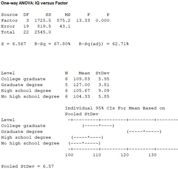
From the MINITAB output, the test valueF is 13.33.

Conclusion:

From the results, the test value is 13.33.

Here, the F-statistic value is greater than the critical value.

That is, 13.33>3.13 .

Thus, it can be concluding that, the null hypothesis is rejected.

Hence, there is evidence to reject the claim thatthe mean IQs of the various educational levels of the subjectsare equal. So use Scheffe test for where the difference exists.

Consider, X¯1 , X¯2 , X¯3 and X¯4 represents the means of No high school degree, High school degree, College graduate and Graduate degree, s12,s22s32 and s42 represents the variances of samples of No high school degree, High school degree, College graduate and Graduate degree.

From the Minitab output, the sample sizes n1,n2,n3 and n4 are 6, 6, 6 and 5.

The means are X¯1,X¯2X¯3 and X¯4 are 104.33, 105.67, 109.83 and 127.00.

The sample variances are s12,s22s32 and s42 are 34.2225, 82.6281, 35.4025 and 14.5161.

Critical value:

The formula for critical value F1 for the Scheffe test is,

F1=(k1)(Critical value)

Here, the critical value of F test is 3.13.

Substitute 3.13 for critical value is of F and 3 for k-1 in F1

F1=3(3.13)=9.39

Comparison of the means:

The formula for finding sW2 is,

sW2=(ni1)si2(ni1)

That is,

sW2=(61)34.2225+(61)82.6281+(61)35.4025+(51)14.5161(61)+(61)+(61)+(51)=171.1125+413.1405+177.0125+58.064419=819.329919=43.1226

Comparison between the means X¯1 and X¯2 :

The hypotheses are given below:

Null hypothesis:

H0: There is no significant difference between X¯1 and X¯2 .

Alternative hypothesis:

H1: There is significant difference between X¯1 and X¯2 .

Rejection region:

The null hypothesis would be rejected if absolute value greater than the critical value.

The formula for comparing the means X¯1 and X¯2 is,

Fs=(X¯1X¯2)2sW2[1n1+1n2]

Substitute 104.33 and 105.67 for X¯1 and X¯2 , 6 for n1, 6 for n2 and 43.1226 for sW2

Fs=(104.33105.67)243.1226[16+16]=1.795643.1226[0.1667+0.1667]=1.795614.3771=0.125

Thus, the value of Fs is 0.125.

Conclusion:

The value of Fs is 0.125.

Here, the value of Fs is lesser than the critical value.

That is, 0.125<9.39 .

Thus, the null hypothesis is not rejected.

Hence, there is no significant difference between the means X¯1 and X¯2 .

Comparison between the means X¯1 and X¯3 :

The hypotheses are given below:

Null hypothesis:

H0: There is no significant difference between X¯1 and X¯3 .

Alternative hypothesis:

H1: There is significant difference between X¯1 and X¯3 .

Rejection region:

The null hypothesis would be rejected if absolute value greater than the critical value.

The formula for comparing the means X¯1 and X¯3 .is,

Fs=(X¯1X¯3)2sW2[1n1+1n3]

Substitute 104.33 and 109.83 for X¯1 and X¯3 , 6 for n1, 6 for n3 and 43.1226 for sW2

Fs=(104.33109.83)243.1226[16+16]=30.2543.1226[0.1667+0.1667]=30.2514.3771=2.104

Thus, the value of Fs is 2.104.

Conclusion:

The value of Fs is 2.104.

Here, the value of Fs is lesser than the critical value.

That is, 2.104<9.39 .

Thus, the null hypothesis is not rejected.

Hence, there is no significant difference between the means X¯1 and X¯3 .

Comparison between the means X¯2 and X¯3 :

The hypotheses are given below:

Null hypothesis:

H0: There is no significant difference between X¯2 and X¯3 .

Alternative hypothesis:

H1: There is significant difference between X¯2 and X¯3 .

Rejection region:

The null hypothesis would be rejected if absolute value greater than the critical value.

The formula for comparing the means X¯2 and X¯3 .is,

Fs=(X¯2X¯3)2sW2[1n2+1n3]

Substitute 105.67 and 109.83 for X¯2 and X¯3 , 6 for n2, 6 for n3 and 43.1226 for sW2

Fs=(105.67109.83)243.1226[16+16]=17.305643.1226[0.1667+0.1667]=17.305614.3771=1.204

Thus, the value of Fs is 1.204.

Conclusion:

The value of Fs is 1.204.

Here, the value of Fs is lesser than the critical value.

That is, 1.204<9.39 .

Thus, the null hypothesis is not rejected.

Hence, there is no significant difference between the means X¯2 and X¯3 .

Comparison between the means X¯1 and X¯4 :

The hypotheses are given below:

Null hypothesis:

H0: There is no significant difference between X¯1 and X¯4 .

Alternative hypothesis:

H1: There is significant difference between X¯1 and X¯4 .

Rejection region:

The null hypothesis would be rejected if absolute value greater than the critical value.

The formula for comparing the means X¯1 and X¯4 .is,

Fs=(X¯1X¯4)2sW2[1n2+1n4]

Substitute 104.33 and 127.00 for X¯1 and X¯4 , 6 for n1, 5 for n4 and 43.1226 for sW2

Fs=(104.33127.00)243.1226[16+15]=513.928943.1226[0.1667+0.2]=513.928915.8131=32.5002

Thus, the value of Fs is 32.5002.

Conclusion:

The value of Fs is 32.5002.

Here, the value of Fs is greater than the critical value.

That is, 32.5002>9.39 .

Thus, the null hypothesis is rejected.

Hence, there is significant difference between the means X¯1 and X¯4 .

Comparison between the means X¯2 and X¯4 :

The hypotheses are given below:

Null hypothesis:

H0: There is no significant difference between X¯2 and X¯4 .

Alternative hypothesis:

H1: There is significant difference between X¯2 and X¯4 .

Rejection region:

The null hypothesis would be rejected if absolute value greater than the critical value.

The formula for comparing the means X¯2 and X¯4 .is,

Fs=(X¯2X¯4)2sW2[1n2+1n4]

Substitute 105.67 and 127.00 for X¯2 and X¯4 , 6 for n2, 5 for n4 and 43.1226 for sW2

Fs=(105.67127.00)243.1226[16+15]=454.968943.1226[0.1667+0.2]=454.968915.8131=28.7716

Thus, the value of Fs is 28.7716.

Conclusion:

The value of Fs is 28.7716.

Here, the value of Fs is greater than the critical value.

That is, 28.7716>9.39 .

Thus, the null hypothesis is rejected.

Hence, there is significant difference between the means X¯2 and X¯4 .

Comparison between the means X¯3 and X¯4 :

The hypotheses are given below:

Null hypothesis:

H0: There is no significant difference between X¯3 and X¯4 .

Alternative hypothesis:

H1: There is significant difference between X¯3 and X¯4 .

Rejection region:

The null hypothesis would be rejected if absolute value greater than the critical value.

The formula for comparing the means X¯3 and X¯4 .is,

Fs=(X¯3X¯4)2sW2[1n3+1n4]

Substitute 109.83 and 127.00 for X¯3 and X¯4 , 6 for n2, 5 for n4 and 43.1226 for sW2

Fs=(109.83127.00)243.1226[16+15]=294.808943.1226[0.1667+0.2]=294.808915.8131=18.6433

Thus, the value of Fs is 18.6433.

Conclusion:

The value of Fs is 18.6433.

Here, the value of Fs is greater than the critical value.

That is, 18.6433>9.39 .

Thus, the null hypothesis is rejected.

Hence, there is significant difference between the means X¯3 and X¯4 .

Justification:

Here, there is significant difference between the means X¯1 and X¯4 , X¯2 and X¯4 , and X¯3 and X¯4 . Thus, it can be concluding that there is significant difference between the means of “No high school degree and Graduate degree”, “High school degree and Graduate degree”, “College graduate and Graduate degree”.

Want to see more full solutions like this?

Subscribe now to access step-by-step solutions to millions of textbook problems written by subject matter experts!

Chapter 12 Solutions

ELEMENTARY STATISTICS CONNECT CODE>CUS

Ch. 12.1 - For Exercises 7 through 20, assume that all...Ch. 12.1 - Prob. 11ECh. 12.1 - For Exercises 7 through 20, assume that all...Ch. 12.1 - For Exercises 7 through 20, assume that all...Ch. 12.1 - For Exercises 7 through 20, assume that all...Ch. 12.1 - Prob. 15ECh. 12.1 - For Exercises 7 through 20, assume that all...Ch. 12.1 - For Exercises 7 through 20, assume that all...Ch. 12.1 - For Exercises 7 through 20, assume that all...Ch. 12.1 - For Exercises 7 through 20, assume that all...Ch. 12.1 - For Exercises 7 through 20, assume that all...Ch. 12.2 - Colors That Make You Smarter The following set of...Ch. 12.2 - What two tests can be used to compare two means...Ch. 12.2 - Explain the difference between the two tests used...Ch. 12.2 - For Exercises 3 through 8, the null hypothesis was...Ch. 12.2 - For Exercises 3 through 8, the null hypothesis was...Ch. 12.2 - For Exercises 3 through 8, the null hypothesis was...Ch. 12.2 - For Exercises 3 through 8, the null hypothesis was...Ch. 12.2 - For Exercises 3 through 8, the null hypothesis was...Ch. 12.2 - For Exercises 3 through 8, the null hypothesis was...Ch. 12.2 - For Exercises 9 through 13, do a complete one-way...Ch. 12.2 - Prob. 10ECh. 12.2 - For Exercises 9 through 13, do a complete one-way...Ch. 12.2 - For Exercises 9 through 13, do a complete one-way...Ch. 12.2 - Prob. 13ECh. 12.2 - Prob. 14ECh. 12.3 - Automobile Sales Techniques The following outputs...Ch. 12.3 - Prob. 1ECh. 12.3 - Explain what is meant by main effects and...Ch. 12.3 - Prob. 3ECh. 12.3 - How are the F test values computed?Ch. 12.3 - Prob. 5ECh. 12.3 - In a two-way ANOVA, variable A has six levels and...Ch. 12.3 - Prob. 7ECh. 12.3 - When can the main effects for the two-way ANOVA be...Ch. 12.3 - Prob. 9ECh. 12.3 - For Exercises 9 through 15, perform these steps....Ch. 12.3 - For Exercises 9 through 15, perform these steps....Ch. 12.3 - For Exercises 9 through 15, perform these steps....Ch. 12.3 - Prob. 13ECh. 12.3 - For Exercises 9 through 15, perform these steps....Ch. 12.3 - Prob. 15ECh. 12 - If the null hypothesis is rejected in Exercises 1...Ch. 12 - Prob. 12.1.2RECh. 12 - Prob. 12.1.3RECh. 12 - Prob. 12.1.4RECh. 12 - Prob. 12.1.5RECh. 12 - If the null hypothesis is rejected in Exercises 1...Ch. 12 - Prob. 12.1.7RECh. 12 - Prob. 12.1.8RECh. 12 - Review Preparation for Statistics A statistics...Ch. 12 - Effects of Different Types of Diets A medical...Ch. 12 - Prob. 1DACh. 12 - Prob. 2DACh. 12 - Prob. 3DACh. 12 - Prob. 1CQCh. 12 - Prob. 2CQCh. 12 - Prob. 3CQCh. 12 - Determine whether each statement is true or false....Ch. 12 - Prob. 5CQCh. 12 - Prob. 6CQCh. 12 - Prob. 7CQCh. 12 - Prob. 8CQCh. 12 - Complete the following statements with the best...Ch. 12 - Prob. 10CQCh. 12 - For Exercises 11 through 17, use the traditional...Ch. 12 - Prob. 12CQCh. 12 - Prob. 13CQCh. 12 - Prob. 14CQCh. 12 - Prob. 15CQCh. 12 - Prob. 16CQCh. 12 - For Exercises 11 through 17, use the traditional...Ch. 12 - Shown here are the abstract and two tables from a...Ch. 12 - Shown here are the abstract and two tables from a...Ch. 12 - Prob. 3CTCCh. 12 - Prob. 4CTCCh. 12 - Prob. 5CTCCh. 12 - Prob. 6CTCCh. 12 - Prob. 7CTCCh. 12 - Adult Children of Alcoholics Shown here are the...Ch. 12 - Prob. 9CTCCh. 12 - Prob. 10CTCCh. 12 - Prob. 11CTC
Knowledge Booster
Background pattern image
Statistics
Learn more about
Need a deep-dive on the concept behind this application? Look no further. Learn more about this topic, statistics and related others by exploring similar questions and additional content below.
Recommended textbooks for you
Text book image
Glencoe Algebra 1, Student Edition, 9780079039897...
Algebra
ISBN:9780079039897
Author:Carter
Publisher:McGraw Hill
Statistics 4.1 Introduction to Inferential Statistics; Author: Dr. Jack L. Jackson II;https://www.youtube.com/watch?v=QLo4TEvBvK4;License: Standard YouTube License, CC-BY