
(a)
The IS curve of the economy.
(a)
Explanation of Solution
The investment function of the economy is given by
The values of C, T, I, and G can be substituted into the IS equation as follows:
Thus, the IS curve of the economy can be graphed by plotting the Y value on the horizontal axis as 3000 and r ranging from 0 to 8 as follows:
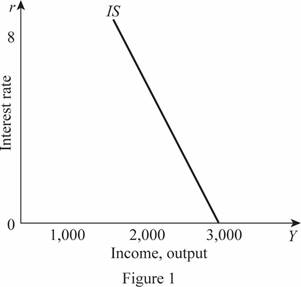
In Figure 1, the horizontal axis measures the income or output and the vertical axis measures the interest rate.
Fiscal policy: The fiscal policy is a policy of the government regarding the government expenditures and taxes of the economy.
(b)
The LM curve of the economy.
(b)
Explanation of Solution
The money demand function of the economy is given to be
The supply of real money balance can be calculated by dividing the money supply by the price level in the economy. Since their values are given, the value of the supply of the real money balance can be calculated as follows:
Thus, the supply of real money balance is 1,000. The LM curve can be calculated by setting the demand equation equal to the supply equation as follows:
Thus, the LM curve with the value of r ranging from 0 to 8 can be plotted as follows:
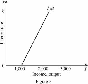
In Figure 2, the horizontal axis measures the income or output and the vertical axis measures the interest rate.
(c)
The IS-LM equilibrium.
(c)
Explanation of Solution
The IS-LM equilibrium can be calculated by equating the IS equation and the LM equation. The IS equation is calculated to be
Substituting the value of r in any equation can provide the value of Y as follows:
Thus, the rate of interest and Y are 5 and 2,000, respectively. These values can be obtained through the graph as follows:
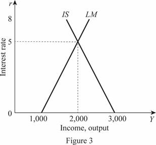
In Figure 3, the horizontal axis measures the income or output and the vertical axis measures the interest rate. The market is in equilibrium at the point where the IS curve intersects with the LM curve.
(d)
The impact of increased government purchases from 500 to 700 on IS and IS-LM equilibrium.
(d)
Explanation of Solution
The values of C, T, I, and G can be substituted into the IS equation as follows:
The new IS curve is 500 more than the previous IS curve, which means that the IS curve will shift toward the right by the value of 500 when the government purchases increases from 500 to 700. Thus, the IS and the LM equations can be equated to calculate the IS-LM equation as follows:
Substituting the value of r in any equation can provide the value of Y as follows:
Thus, the rate of interest and Y are 6.25 and 2,250, respectively. These values can be obtained through the graph as follows:
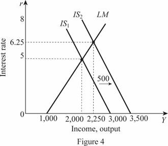
In Figure 4, the horizontal axis measures the income or output and the vertical axis measures the interest rate. Thus, with an increase in the government expenditure from 500 to 700, the IS curve shifts to the right. The equilibrium rate of interest in the economy increases by 1.25 from 5 to 6.25. The change in the income is by $250 and from $2,000, it becomes $2,250.
(e)
The impact of increased money supply from 3000 to 4500 on IS and IS-LM equilibrium.
(e)
Explanation of Solution
The supply of real money balance can be calculated by dividing the money supply by the price level in the economy. Since their values are given, the value of the supply of the real money balance can be calculated as follows:
Thus, the supply of real money balance is 1,500. The LM curve can be calculated by setting the demand equation equal to the supply equation as follows:
Thus, the LM value will change by 500, which means there will be a rightward shift in the LM curve with the value of 500. The rightward shift in the LM curve will lead to the change in the equilibrium and this can be calculated as follows:
Substituting the value of r in any equation can provide the value of Y as follows:
Thus, the rate of interest and Y are 3.75 and 2,250, respectively. These values can be obtained through the graph as follows:
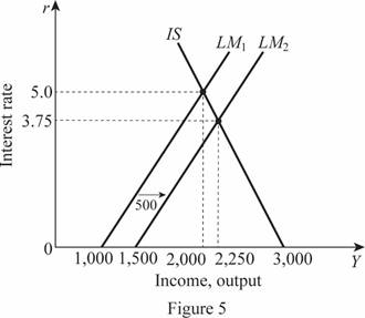
In Figure 5, the horizontal axis measures the income or output and the vertical axis measures the interest rate.
(f)
The impact of increased price level from 3 to 5 on IS and IS-LM equilibrium.
(f)
Explanation of Solution
The supply of real money balance can be calculated by dividing the money supply by the price level in the economy. Since their values are given, the value of the supply of the real money balance can be calculated as follows:
Thus, the supply of real money balance is 600. The LM curve can be calculated by setting the demand equation equal to the supply equation as follows:
Thus, the LM value will change by -400, which means there will be a leftward shift in the LM curve with the value of 400. The leftward shift in the LM curve will lead to the change in the equilibrium and this can be calculated as follows:
Substituting the value of r in any equation can provide the value of Y as follows:
Thus, the rate of interest and Y are 6 and 1,800, respectively. These values can be obtained through the graph as follows:
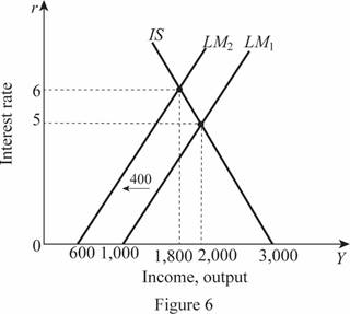
In Figure 6, the horizontal axis measures the income or output and the vertical axis measures the interest rate.
(g)
The impact of changes in the fiscal and monetary policies on aggregate demand.
(g)
Explanation of Solution
The aggregate demand curve is the relationship between the price level in the economy and the level of income of the economy. Thus, the aggregate demand curve can be derived by summating the IS and LM curves and solving it for the value of Y as the function of P. This can be done as follows:
The IS curve can be written in terms of the rate of interest as follows:
Similarly, the LM equation can be written in terms of the rate of interest as follows:
Now, the IS and LM curves can be combined to eliminate the rate of interest and solving the equation for Y as a function of P as follows:
The nominal money supply is given to be 3,000, which can be substituted in the above equation for M and can be calculated as follows:
This aggregate demand equation can be graphed as follows:
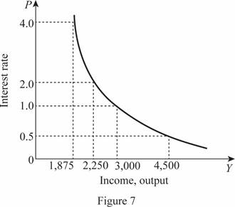
In Figure 7, the horizontal axis measures the income or output and the vertical axis measures the price level. When there is a change in the money supply as well as in the government purchases, the IS curve will be derived with the changed government purchases. This can be calculated as follows:
The IS curve can be written in terms of the rate of interest as follows:
Similarly, the LM equation can be written in terms of the rate of interest as follows:
Now, the IS and LM curves can be combined to eliminate the rate of interest and solving the equation for Y as a function of P as follows:
Thus, the change in the government expenditure with 200 leads to an increase in the aggregate demand with a value of 250. When the expansionary monetary policy increases the money supply from 3,000 to 4,500, the LM curve will change and the new aggregate demand can be calculated as follows:
The normal AD curve is calculated to be
Thus, an increased money supply leads to a rightward shift in the AD curve of the economy.
Want to see more full solutions like this?
Chapter 12 Solutions
MACROECONOMICS+SAPLING+6 M REEF HC>IC<

- The consumption function is given by: C = 200+0.75 (Y-T). I = 200-25r. G = T=100 The money demand function in the Malakas Country is Md = Y-100r. The Money supply M is 1000 and price is 2. For this economy graph the LM curve for ranging from 0 to 8.arrow_forward(Please solve part a) Consider the economy of Hicksonia a) The consumption function is given by: C=300+0.6(Y-T). The investment function is: I=700-80r. Government purchases and taxes are both 500. For this economy, graph the IS curve for r changing from 0 to 8 b) The money demand function in Hicksonia is (M/P)^d=Y-200r. The money supply M is 3000 and the price level P is 3. For this economy, graph the LM curve for r changing from 0 to 8. c) Find the equilibrium interest rate r and the equilibrium level of income Y. d) Suppose that government purchases are increased from 500 to 700. How does the IS curve shift? What are the new equilibrium interest rate and level of income? e) Suppose instead that the money supply is raised from 3000 to 4500. How does the LM cruve shift? What are the new eqquilibrium interest rate and level of income? f) With the initial level values for monetary and fiscal policy, suppose that the price level rises from 3 to 5. What hpapnes? What are the new…arrow_forwardConsider an economy described by the following equations:Y = C + I + G (1)C = 100 + 0.75(Y − T) (2)I = 500 – 50 r (3)G = 125T = 100where Y is GDP, C is consumption, I is investment, G is government purchases, T is taxes, and r is the interest rate. If the economy were at full employment (that is, at its natural rate), GDP would be 2,000.1. Suppose the central bank’s policy is to adjust the money supply to maintain the interest rate at 4 percent, so r = 4. Solve for GDP. Is it greater or lower than full-employment level? How much 2. Assuming no change in monetary policy (as was in part i), what change in government purchases would restore full employment?1. Assuming no change in fiscal policy, what change in the interest rate would restore full employment?arrow_forward
- Economist will focus on achieving macroeconomic goals. There are four major economic goals namely as full employment, price stability, economic growth and equitable distribution of income. However, it is impossible for a government to achieve all four macroeconomic goals simultaneously. Briefly discuss how a government will not be able to implement two particular goals at the same time. According to Keynes, people have demand for money due to three different motives foe holding money rather than other forms. Hence, identify the THREE (3) motives according to Keynesian approach.arrow_forwardConsider the following closed economy in the context of the IS-LM model. The consumption function (C), the investment function (I), government purchases (G), taxes (T), the money demand function (MD), money supply (M) and the price level (P) are given as: C = 500 + 0.75(Y - T)I = 1000 - 300?G = 1000T = 1200MD = 0.5Y - 200rM = 5000P = 2 (a) Write down the equations for the IS curve and LM curve. Show your workings. (b) Solve for the short-run equilibrium output and interest rate. (c) Suppose government purchases falls, with ΔG=-175. (i) Using the Keynesian cross model, calculate the change in equilibrium output. (Hint: Use the government purchases multiplier.) (ii) Would your answer be the same if you calculate the change in equilibrium output using the IS-LM model? Briefly explain your answer. (e) Suppose the price level falls. Using an appropriate IS-LM diagram, illustrate the short-run impact of the fall in price level on the equilibrium interest rate and output. No written…arrow_forwardanswer c and d Suppose that the following system of equations describe the macroeconomy of a hypothetical country: Y= C(y)+I(i)+G : IS or goods market M/p=L(i,y) : LM or money market b) Taking money supply and government expenditure as exogenous and the price level as fixed, determine and provide economic intuition for the signs and magnitudes of the following multipliers dY/dG and di/dG c) For a simultaneous increase in both the interest elasticity of investment and interest elasticity demand for money parameters, determine the net effect on the values of the multipliers in part b). d) For a horizontal LM curve, determine the numerical values of your answers in part b) above if: Marginal propensity to consume=5/6 Tax rate=0.25 Interest elasticity of investment=5 Interest elasticity of demand for money=50 Income elasticity of demand for money=2 answer c and d onlyarrow_forward
- Assume that the money demand function is (M / P) ^ d = 2, 200 - 200r, where r is the interest rate in percent. The money supply M is 2,000 and the price level P is 2. The consumption function is given by C = 200 + 0.5(Y - T) and the investment function is I = 1.000 - 200r , where r is measured in percent , G equals 300, and T equals 200. Calculate the equilibrium level of output. Show the IS-LM equilibrium graphically.arrow_forwardDiscuss the impact of monetary and fiscal policy in each of these special cases:4. 1.1. If investment does not depend on the interest rate, the IS curve is vertical.4.1.2. If money demand does not depend on the interest rate, the LM curve is vertical.arrow_forward111.If money demand does not depend on income, then the ______ curve is ______. A)IS; vertical B)IS; horizontal C)LM; vertical D)LM; horizontal 112.If money demand is extremely sensitive to the interest rate, then the ______ curve is ______. A)IS; vertical B)IS; horizontal C)LM; vertical D)LM; horizontal 113.If the government wants to raise investment but keep output constant, it should: A)adopt a loose monetary policy but keep fiscal policy unchanged. B)adopt a loose monetary policy and a loose fiscal policy. C)adopt a loose monetary policy and a tight fiscal policy. D)keep monetary policy unchanged but adopt a tight fiscal policy. 114.A tax cut combined with tight money, as was the case in the United States in the early 1980s, should lead to a: A)rise in the real interest rate and a fall in investment. B)fall in the real interest rate and a rise in investment. C)rise in both the real interest rate and investment. D)fall in both the real interest…arrow_forward
- Policymakers aim at increasing output Y, but keeping the interest rate, i, constant. Which of the following policy mix can achieve this target?All of the answers here are incorrect.A combination of increasing G and increasing the money supply.A combination of increasing G and maintaining the money supply unchanged.A combination of decreasing G and decreasing the money supply.A combination of increasing G and decreasing the money supply.arrow_forwardDetermine whether each of the following statements is true or false, and explain why. For each true statement, discuss the impact of monetary and fiscal policy in that special case. a) If money demand does not depend on income, the LM curve is horizontal. b) If money demand is extremely sensitive to the interest rate, the LM curve is horizontal.arrow_forwardIn a small closed economy, its aggregate demand and output are given as the equations below, Y = C + I + G; national output or GDP. C = 100 + 0.5(Y-T); consumption, marginal propensity to consume MPC = 0.5. I = 150 – 10*r; investment is a negative function of real interest rate (r as %). (M/P)d = Y – 20*r; real money demand which is adjusted by price level (inflation). G = 200; as government spending. T = 200; as tax. M = 2,400; as money supply. P = 4; the price level. (1) With the equations above, try to derive the IS curve. Tip: recall IS curve represent the relation between national output (Y) and real interest rate (r) in goods market. To derive IS curve, you need to put all components of Y together and find its connection with r. (2) Use the same equations, now try to derive the LM curve. Tip: recall LM curve represent the relation between national output (Y) and real interest rate (r) in money market. So to derive LM curve, you need to consider money supply and demand.…arrow_forward


 Economics (MindTap Course List)EconomicsISBN:9781337617383Author:Roger A. ArnoldPublisher:Cengage Learning