Chapter 12, Problem 55CE

Instructions: Choose one or more of the data sets A-J below, or as assigned by your instructor. The first column is X, or independent, variable and the second column is the Y, or dependent, variable. Use Excel or a statistical package (e.g., MegaStat or Minitab) to obtain the simple regression and required graphs. Write your answers to exercises 12.46 through 12.61 (or those assigned by your instructor) in a concise report, labeling your answers to each question. Insert tables and graphs in your report as appropriate. You may work with a partner if your instructor allows it.

(a) Based on the R² and ANOVA table for your model, how would you assess the fit? (b) Interpret the p-value for the F statistic. (c) Would you say that your model’s fit is good enough to be of practical value?

DATA SET B Midterm and Final Exam Scores for Business Statistics Students, Fall Semester 2011 (n = 58 students)

To determine

Explain how one would assess the fit based on the $R^2$ and ANOVA table.

Explanation of Solution

Answer will vary.

Here the data set B is taken, in which the midterm exam (X) and final exam score (Y) is given.

Hypotheses:

Null hypothesis:

$H_0:{\beta }_1=0$

That is, the slope is zero.

Alternative hypothesis:

$H_1:{\beta }_1\ne 0$

That is, the slope not equal to zero.

Regression:

Suppose $x_1\mathrm{...}{x}_n$ be n sample values of independent variable and the corresponding dependent variable values are $y_1\mathrm{...}{y}_n$. The slope and the intercept of ordinary least square can be defined as $b_0=\overline{y}-b_1\overline{x}$ and $b_1=\frac{S{S}_{xy}}{S{S}_{xx}}$.

Where, $S{S}_{xx},S{S}_{yy},S_{xy}$ are the sum of squares due to x, y and xy respectively. $\overline{x}\text{and}\overline{y}$ are the sample mean of the independent and dependent variable respectively.

The total sum of squares is denoted as, $SST={\displaystyle \sum _{i=1}^n\left(y_i-\overline{y}\right)}$.

The regression sum of squares is denoted as, $SSR={\displaystyle \sum _{i=1}^n\left({\widehat{y}}_i-\overline{y}\right)}$.

The error sum of squares is denoted as, $SSE={\displaystyle \sum _{i=1}^n{\left(y_i-{\widehat{y}}_i\right)}^2}$.

From the regression the fitted line is denoted as, $\widehat{y}=b_0+b_{1}x$ .

The 95% confidence interval for the slope, ${\beta }_1$ is defined as,

$b_1-t_{\frac{\alpha }{2}}{s}_{b_1}\le {\beta }_1\le b_1+t_{\frac{\alpha }{2}}{s}_{b_1}$

Where, $b_1$ is the slope, $t_{\frac{\alpha }{2}}$ be the table value of t-distribution for two-tailed with $\alpha$ level of significance and $s_{b_1}$ is the standard error of the slope denoted as, $s_{b_1}=\frac{s_e}{\sqrt{{\displaystyle \sum _{i=1}^n\left(x_i-\overline{x}\right)}}},s_e\text{ is the standard error}\text{.}$$s_e=\sqrt{\frac{SSE}{n-2}}$ with sample size n and the sum of squares due to error.

Software Procedure:

Step-by-step software procedure to find R-squared using EXCEL is as follows:

• • Open an EXCEL file.
• • In column A and B, the Midterm Exam Score and Final Exam Score data were entered.
• • Click on data > click on Data analysis.
• • Choose Regression > click OK.
• • Select Input Y range asthe column of Final Exam Score.
• • Select Input X range asthe column of Midterm Exam Score.
• • Select the output range.
• • Click OK.
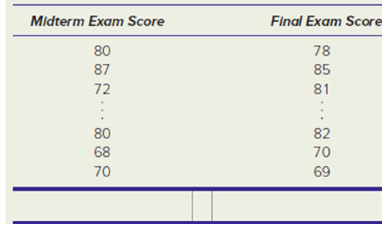
• Output using EXCEL is given below:

From the output, the R-squared value is 0.429.

$R^2$(R-squared):

The coefficient of determination ($R^2$) is defined as the proportion of variation in the observed values of the response variable that is explained by the regression. The squared correlation gives fraction of variability of response variable (y) accounted for by the linear regression model.

The $R^2$ value is 42.9%, which means that the percentage of variation in the observed values of final exam score that is explained by the regression is 42.9%. That is, only 42.9% of the variability in final exam score is explained by the midterm exam scores with a linear relationship.

To determine

Interpret the p-value for the F statistic.

Explanation of Solution

Calculation:

For the F-test of the slope the p-value is 0.000.

Decision rule:

If $p\text{-value}\le \alpha$, reject the null hypothesis.

If $p\text{-value >}\alpha$, fail to reject the null hypothesis.

It is assumed that the level of significance is 0.05.

Conclusion:

Here the p-value is less than the level of significance.

That is, $0.000\left(=p\text{-value}\right)<0.05\left(=\alpha \right)$ .

Hence, by the decision rule, reject the null hypothesis.

Therefore, it can be concluded that there is not sufficient evidence to support that the slope is zero.

Hence, the linear model provides significant fit.

To determine

Check whether the model’s fit is good enough to be of practical value.

Explanation of Solution

Now, a hypothesis test is needed to check the whether the model provides good fit or not.

Decision rule:

If $F_{cal}>F_{1,n-2}$, reject the null hypothesis.

If $F_{cal}\le F_{1,n-2}$, fail to reject the null hypothesis.

Critical value:

Here from the output, the sample size, $n=58$.

The degrees of freedom is,

$\begin{array}{c}df=n-2\\ =58-2\\ =56\end{array}$

Thus, the degrees of freedom is56.

For two tailed test, the critical value for t-test will be, $F_{1,n-2}$.

It is assumed that the level of significance, $\alpha =0.05$.

Procedure for critical-value using EXCEL:

Software Procedure:

Step-by-step software procedure to obtain critical-value using EXCEL software is as follows:

• • Open an EXCEL file.
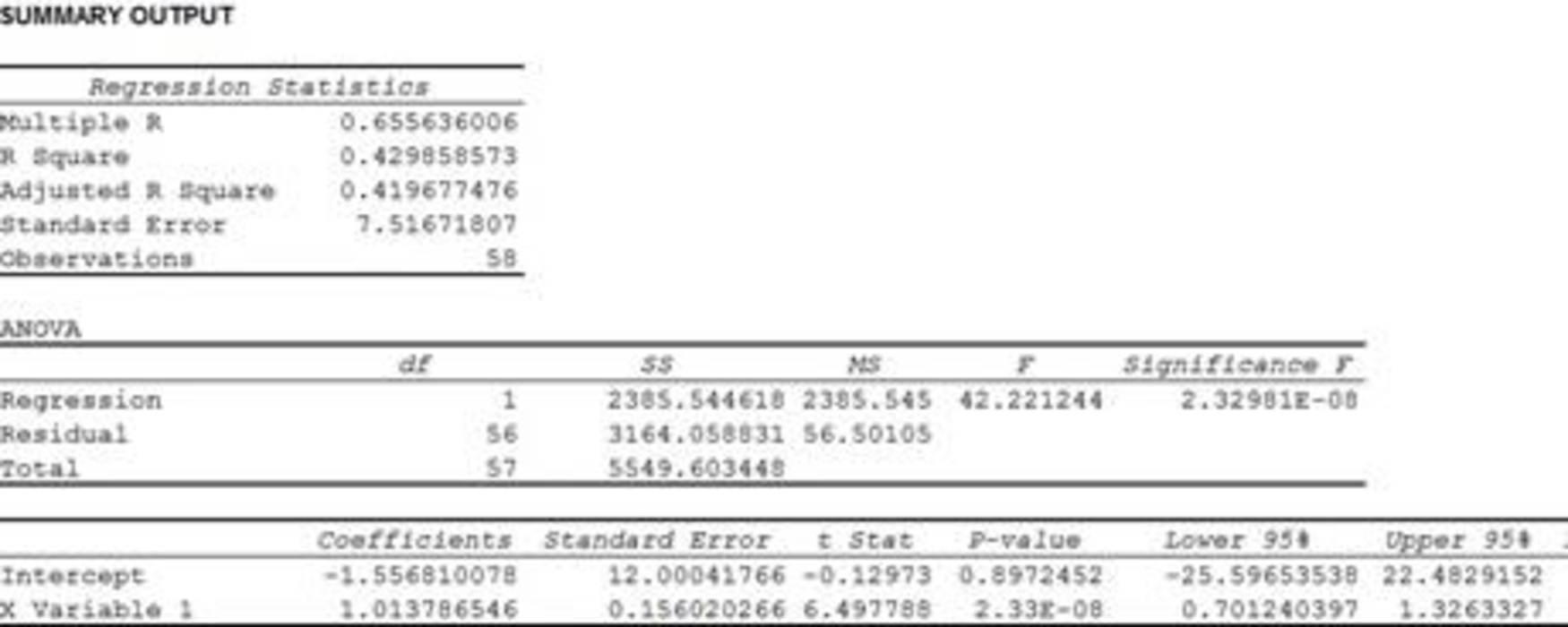
• • In cell A1, enter the formula “=F.INV.RT(0.05,1,56)”
• Output using EXCEL software is given below:

Hence, the critical value will be 4.013.

From the output of part (a), the F-statistic value is 42.22.

The level of significance is 0.05.

Conclusion:

Here the F-statistics is greater than the critical value.

That is, $F-\text{statistics}\left(=42.22\right)\text{> Critical value}\left(=4.013\right)$ .

Hence, by the decision rule, reject the null hypothesis.

Therefore, it can be concluded that there is not sufficient evidence to support that the slope is zero.

Hence, linear model provides significant fit.

The coefficient of determination ($R^2$) measures the overall fit of the regression. However, here the value of the $R^2$ (= 0.43) is not near to 1.

Thus, using $R^2$ the model’s fit is not good enough to be of practical value.