Chapter 12.7, Problem 30P

Use γ-ϕ approach to model the vapor-liquid equilibrium of an ethyne [acetylene] (1) + 1, 1 difluoro ethane [R-152a] (2) system at 303.2 K. Treat the

liquid using the 2-parameter Margules equation and the vapor as an ideal solution (described by the virial equation). Report the following:

• Raoult’s Law predictions
• Modified Raoult’s Law predictions (ideal gas for the vapor phase)
• γ-ϕ modeling results Experimental data as symbols given in Table P12-30

Table P12-30 Vapor-liquid equilibrium of ethyne (1) + R-152a (2) at 303.2K.

Interpretation Introduction

Interpretation:

Using gamma phi modelling approach, predict the $P_{xy}$ diagram for the system using the two parameter Wilson equation and the virial equation.

Concept Introduction:

Write the Antoine equation for the component.

${\log }_{10}\left(P_1{}^{sat}\right)=A-\frac{B}{T+C}$

Write the expression to calculate the parameter $a$ for component.

$a=\frac{27R^2{T}_c{}^2}{64P_c}$

Here, gas constant is $R$, critical temperature and critical pressure for component are $T_c$ and $P_c$ respectively.

Write the expression to calculate the parameter $b$ for component.

$b=\frac{R{T}_c}{8P_c}$

Write the expression for the van Laar parameters.

$L_{12}=\frac{b_1}{RT}{\left(\frac{\sqrt{a_1}}{b_1}-\frac{\sqrt{a_2}}{b_2}\right)}^2$

$L_{21}=\frac{b_2}{RT}{\left(\frac{\sqrt{a_1}}{b_1}-\frac{\sqrt{a_2}}{b_2}\right)}^2$

Here, temperature is T, parameters of the van Laar equation using the VDW definitions is $L_{12},L_{21}$, and equation of state parameter $a_1,b_1,a_2,\text{and}{b}_2$.

Write the activity coefficients from the van Laar model for components 1 and 2.

$\ln \left[{\gamma }_1\right]=L_{12}{\left(1+\frac{L_{12}{x}_1}{L_{21}{x}_2}\right)}^{-2}$

$\ln \left[{\gamma }_2\right]=L_{21}{\left(1+\frac{L_{21}{x}_2}{L_{12}{x}_1}\right)}^{-2}$

Here, liquid phase mole fraction for component 1 and 2 is $x_1\text{and}{x}_2$ respectively.

Write the expression to calculate the value of ${B^{\prime }}_1$.

$\begin{array}{c}{B^{\prime }}_1=\frac{\left(B^0+{\omega }_1{B}^1\right)R{T}_{c,1}}{P_{c,1}}\\ =\frac{\left[\left(0.083-\frac{0.422}{T_{r,1}^{1.6}}\right)+{\omega }_1\left(0.139-\frac{0.172}{T_{r,1}^{4.2}}\right)\right]R{T}_{c,1}}{P_{c,1}}\end{array}$

Here, reduced temperature of component 1 is $T_{r,1}$, acentric factor of component 1 is ${\omega }_1$, and second virial coefficients are $B^0\text{and}{B}^1$.

Write the expression to calculate the value of ${B^{\prime }}_2$.

$\begin{array}{c}{B^{\prime }}_2=\frac{\left(B^0+{\omega }_2{B}^1\right)R{T}_{c,2}}{P_{c,2}}\\ =\frac{\left[\left(0.083-\frac{0.422}{T_{r,2}^{1.6}}\right)+{\omega }_2\left(0.139-\frac{0.172}{T_{r,2}^{4.2}}\right)\right]R{T}_{c,2}}{P_{c,2}}\end{array}$

Here, reduced temperature of component 1 is $T_{r,1}$, acentric factor of component 1 is ${\omega }_1$, and second virial coefficients are $B^0\text{and}{B}^1$.

Write the expression to calculate the fugacity coefficient of component 1$\left({\widehat{\phi }}_{1,sat}\right)$.

$\ln \left({\widehat{\phi }}_{1,sat}\right)=\frac{P_1^{sat}{B^{\prime }}_1}{RT}$

Write the expression to calculate the fugacity coefficient of component 2$\left({\widehat{\phi }}_{2,sat}\right)$.

$\ln \left({\widehat{\phi }}_{2,sat}\right)=\frac{P_2^{sat}{B^{\prime }}_2}{RT}$

Write the expression for Raoult’s law equation.

$P=x_1{P}_1^{sat}+x_2{P}_2^{sat}$

$y_1=\frac{x_1{P}_1^{sat}}{P}$

Write the expression for the vapor definitions of the fugacity coefficients for component 1 and 2.

$\ln \left({\widehat{\phi }}_1\right)=\frac{P}{RT}\left[{B^{\prime }}_{11}+y_2^2\left(2{B^{\prime }}_{12}-{B^{\prime }}_{11}-{B^{\prime }}_{22}\right)\right]$

$\ln \left({\widehat{\phi }}_2\right)=\frac{P}{RT}\left[{B^{\prime }}_{22}+y_1^2\left(2{B^{\prime }}_{12}-{B^{\prime }}_{11}-{B^{\prime }}_{22}\right)\right]$

Here, system pressure is P, vapor phase mole fraction for components 1 and 2 is $y_1\text{and}{y}_2$, second-virial coefficient of component 1 interacting with component 2 is ${B^{\prime }}_{12}$,

second-virial coefficient of pure component 1 and 2 is ${B^{\prime }}_{11}\text{and}{B^{\prime }}_{22}$ respectively.

Write the 2-parameter Margules equation.

$\ln \left({\gamma }_1^{\infty }\right)=A_{12}$

$\ln \left({\gamma }_2^{\infty }\right)=A_{21}$

Here, coefficient of 2-parameter Margules equation is $A_{12}\text{and}{A}_{21}$ respectively.

Write the excess molar Gibbs free energy for model.

$\frac{{\underset{\_}{G}}^E}{RT}=x_1{x}_2\left(A_{21}{x}_1+A_{12}{x}_2\right)$

Write the excess molar Gibbs free energy for experimental.

$\frac{{\underset{\_}{G}}^E}{RT}=x_1\ln \left[{\gamma }_1\right]+x_2\ln \left[{\gamma }_2\right]$

Write the objective function value.

$\text{OBJ}=\frac{1}{N}{{\displaystyle \sum _{i=1}^N\left[\frac{{\left(\frac{{\underset{\_}{G}}^E}{RT}\right)}_i^{Model}-{\left(\frac{{\underset{\_}{G}}^E}{RT}\right)}_i^{Exp}}{{\left(\frac{{\underset{\_}{G}}^E}{RT}\right)}_i^{Exp}}\right]}}^2$

Here, total number of data point is N.

Explanation of Solution

Referring to Appendix C.1, “Critical point, enthalpy of phase change, and liquid molar volume”, obtains the critical temperature, critical pressure and acentric factor of Acetylene (1) and 1,1 Difluroethane (2) as in Table (1).

Compound	Critical temperature $T_c\left(\text{K}\right)$	Reduced temperature $T_r\left(\text{K}\right)$	Critical pressure $P_c\left(\text{bar}\right)$	Acentric factor $\left(\omega \right)$	Liquid molar volume ${\underset{\_}{V}}^L\left({\text{m}}^{\text{3}}/\text{mol}\right)$
Acetylene (1)	308.3	0.9834	61.14	0.189	$43.47\times {10}^{-6}$
Difluroethane (2)	386.41	0.7846	45.17	0.275	$74.51\times {10}^{-6}$

Referring to Appendix E, “Antoine Coefficients”, obtain the constants A, B, and C for component (1) as 4.66141, 909.079, and 7.947 respectively.

Calculate the Antoine equation for the component propane (1).

${\log }_{10}\left(P_1{}^{sat}\right)=A-\frac{B}{T+C}$        (1)

Substitute $30.05°\text{C}$ for T, 4.66141 for A, 909.079 for B, and 7.947 for C in Equation (1).

$\begin{array}{l}{\log }_{10}\left(P_1{}^{sat}\right)=4.66141-\frac{909.079}{7.947+30.05}\\ P_1^{sat}={10}^{-19.2636}\\ P_1^{sat}=5.4499\times {10}^{-20}\text{mmHg}\times \frac{1\text{bar}}{750.06\text{mmHg}}\\ P_1^{sat}=7.26\times {10}^{-23}\text{bar}\end{array}$

Refer the Appendix E, “Antoine Coefficients”, obtain the constants A, B, and C for component as 7.03000, 910.000, and 244.000 respectively.

Calculate the Antoine equation for the component (2).

${\log }_{10}\left(P_2{}^{sat}\right)=A-\frac{B}{T+C}$        (2)

Substitute $\text{30}\text{.05°C}$ for T, 7.03 for A, 910.0 for B, and 244.0 for C in Equation (2).

$\begin{array}{l}{\log }_{10}\left(P_2{}^{sat}\right)=7.03-\frac{910.0}{\text{30}\text{.05°C}+244}\\ P_2{}^{sat}={10}^{3.709}\\ =5121.98\text{mmHg}\times \frac{1\text{bar}}{750.06\text{mmHg}}\\ =6.828\text{bar}\end{array}$

Calculate the parameter $a_1$ for component 1.

$a_1=\frac{27R^2{T}_{c,1}^2}{64P_{c,1}}$        (3)

Here, critical temperature and critical pressure for component 1 are $T_{c,1}$ and $P_{c,1}$ respectively.

Substitute 308.3 K for $T_{c,1}$, 61.14 bar for $P_{c,1}$, and $8.314\times {10}^{-5}\frac{{\text{m}}^{\text{3}}\cdot \text{bar}}{\text{mol}\cdot \text{K}}$ for R in Equation (3).

$\begin{array}{c}{a}_1=\frac{27{\left(8.314\times {10}^{-5}\frac{{\text{m}}^{\text{3}}\cdot \text{bar}}{\text{mol}\cdot \text{K}}\right)}^2{\left(308.3\text{K}\right)}^2}{64\left(61.14\text{bar}\right)}\\ =4.53\times {10}^{-6}\frac{{\text{m}}^{\text{6}}\cdot \text{bar}}{{\text{mol}}^2}\end{array}$

Calculate the parameter $a_2$ for component 2.

$a_2=\frac{27R^2{T}_{c,2}^2}{64P_{c,2}}$        (4)

Here, critical temperature and critical pressure for component 2 are $T_{c,2}$ and $P_{c,2}$ respectively

Substitute 386.41 K for $T_{c,2}$, 45.17 bar for $P_{c,2}$, and $8.314\times {10}^{-5}\frac{{\text{m}}^{\text{3}}\cdot \text{bar}}{\text{mol}\cdot \text{K}}$ for R in Equation (4).

$\begin{array}{c}{a}_2=\frac{27{\left(8.314\times {10}^{-5}\frac{{\text{m}}^{\text{3}}\cdot \text{bar}}{\text{mol}\cdot \text{K}}\right)}^2{\left(386.41\text{K}\right)}^2}{64\left(45.17\text{bar}\right)}\\ =9.63\times {10}^{-6}\frac{{\text{m}}^{\text{6}}\cdot \text{bar}}{{\text{mol}}^2}\end{array}$

Calculate the parameter $b_1$ for component 1.

$b_1=\frac{R{T}_{c,1}}{8P_{c,1}}$        (5)

Substitute 308.3 K for $T_{c,1}$, 61.14 bar for $P_{c,1}$, and $8.314\times {10}^{-5}\frac{{\text{m}}^{\text{3}}\cdot \text{bar}}{\text{mol}\cdot \text{K}}$ for R in Equation (5).

$\begin{array}{c}{b}_1=\frac{\left(8.314\times {10}^{-5}\frac{{\text{m}}^{\text{3}}\cdot \text{bar}}{\text{mol}\cdot \text{K}}\right)308.3\text{K}}{8\left(61.14\text{bar}\right)}\\ =5.24\times {10}^{-5}\frac{{\text{m}}^{\text{3}}}{\text{mol}}\end{array}$

Calculate the parameter $b_2$ for component 2.

$b_2=\frac{R{T}_{c,2}}{8P_{c,2}}$        (6)

Substitute 386.41 K for $T_{c,2}$, 45.17 bar for $P_{c,2}$, and $8.314\times {10}^{-5}\frac{{\text{m}}^{\text{3}}\cdot \text{bar}}{\text{mol}\cdot \text{K}}$ for R in Equation (6).

$\begin{array}{c}{b}_2=\frac{\left(8.314\times {10}^{-5}\frac{{\text{m}}^{\text{3}}\cdot \text{bar}}{\text{mol}\cdot \text{K}}\right)386.41\text{K}}{8\left(45.17\text{bar}\right)}\\ =8.89\times {10}^{-5}\frac{{\text{m}}^{\text{3}}}{\text{mol}}\end{array}$

Calculate the van Laar parameters $\left(L_{12}\right)$.

$L_{12}=\frac{b_1}{RT}{\left(\frac{\sqrt{a_1}}{b_1}-\frac{\sqrt{a_2}}{b_2}\right)}^2$        (7)

Substitute $8.314\times {10}^{-5}\frac{{\text{m}}^{\text{3}}\cdot \text{bar}}{\text{mol}\cdot \text{K}}$ for R, $30.05°\text{C}$ for T, $4.533\times {10}^{-6}\frac{{\text{m}}^{\text{6}}\cdot \text{bar}}{{\text{mol}}^2}$ for $a_1$, $9.639\times {10}^{-5}\frac{{\text{m}}^{\text{6}}\cdot \text{bar}}{{\text{mol}}^2}$ for $a_2$, $5.240\times {10}^{-5}\frac{{\text{m}}^{\text{3}}}{\text{mol}}$ for $b_1$, and $8.890\times {10}^{-5}\frac{{\text{m}}^{\text{3}}}{\text{mol}}$ for $b_2$ in Equation (7).

$\begin{array}{c}{L}_{12}=\frac{b_1}{RT}{\left(\frac{\sqrt{a_1}}{b_1}-\frac{\sqrt{a_2}}{b_2}\right)}^2\\ =\frac{5.240\times {10}^{-5}\frac{{\text{m}}^{\text{3}}}{\text{mol}}}{\left(8.314\times {10}^{-5}\frac{{\text{m}}^{\text{3}}\cdot \text{bar}}{\text{mol}\cdot \text{K}}\right)30.05°\text{C}}{\left(\begin{array}{l}\frac{\sqrt{4.533\times {10}^{-6}\frac{{\text{m}}^{\text{6}}\cdot \text{bar}}{{\text{mol}}^2}}}{5.240\times {10}^{-5}\frac{{\text{m}}^{\text{3}}}{\text{mol}}}\\ -\frac{\sqrt{9.639\times {10}^{-5}\frac{{\text{m}}^{\text{6}}\cdot \text{bar}}{{\text{mol}}^2}}}{8.890\times {10}^{-5}\frac{{\text{m}}^{\text{3}}}{\text{mol}}}\end{array}\right)}^2\\ =\frac{5.240\times {10}^{-5}\frac{{\text{m}}^{\text{3}}}{\text{mol}}}{\left(8.314\times {10}^{-5}\frac{{\text{m}}^{\text{3}}\cdot \text{bar}}{\text{mol}\cdot \text{K}}\right)\left(30.05+273.15\right)\text{K}}{\left(\begin{array}{l}\frac{\sqrt{4.533\times {10}^{-6}\frac{{\text{m}}^{\text{6}}\cdot \text{bar}}{{\text{mol}}^2}}}{5.240\times {10}^{-5}\frac{{\text{m}}^{\text{3}}}{\text{mol}}}-\\ \frac{\sqrt{9.639\times {10}^{-5}\frac{{\text{m}}^{\text{6}}\cdot \text{bar}}{{\text{mol}}^2}}}{8.890\times {10}^{-5}\frac{{\text{m}}^{\text{3}}}{\text{mol}}}\end{array}\right)}^2\\ =0.067713\end{array}$

Calculate the van Laar parameter $\left(L_{21}\right)$.

$L_{21}=\frac{b_2}{RT}{\left(\frac{\sqrt{a_1}}{b_1}-\frac{\sqrt{a_2}}{b_2}\right)}^2$        (8)

Substitute $8.314\times {10}^{-5}\frac{{\text{m}}^{\text{3}}\cdot \text{bar}}{\text{mol}\cdot \text{K}}$ for R, $30.05°\text{C}$ for T, $4.533\times {10}^{-6}\frac{{\text{m}}^{\text{6}}\cdot \text{bar}}{{\text{mol}}^2}$ for $a_1$, $9.639\times {10}^{-5}\frac{{\text{m}}^{\text{6}}\cdot \text{bar}}{{\text{mol}}^2}$ for $a_2$, $5.240\times {10}^{-5}\frac{{\text{m}}^{\text{3}}}{\text{mol}}$ for $b_1$, and $8.890\times {10}^{-5}\frac{{\text{m}}^{\text{3}}}{\text{mol}}$ for $b_2$ in Equation (8).

$\begin{array}{c}{L}_{21}=\frac{b_2}{RT}{\left(\frac{\sqrt{a_1}}{b_1}-\frac{\sqrt{a_2}}{b_2}\right)}^2\\ =\frac{8.890\times {10}^{-5}\frac{{\text{m}}^{\text{3}}}{\text{mol}}}{\left(8.314\times {10}^{-5}\frac{{\text{m}}^{\text{3}}\cdot \text{bar}}{\text{mol}\cdot \text{K}}\right)30.05°\text{C}}{\left(\begin{array}{l}\frac{\sqrt{4.533\times {10}^{-6}\frac{{\text{m}}^{\text{6}}\cdot \text{bar}}{{\text{mol}}^2}}}{5.240\times {10}^{-5}\frac{{\text{m}}^{\text{3}}}{\text{mol}}}\\ -\frac{\sqrt{9.639\times {10}^{-5}\frac{{\text{m}}^{\text{6}}\cdot \text{bar}}{{\text{mol}}^2}}}{8.890\times {10}^{-5}\frac{{\text{m}}^{\text{3}}}{\text{mol}}}\end{array}\right)}^2\\ =\frac{8.890\times {10}^{-5}\frac{{\text{m}}^{\text{3}}}{\text{mol}}}{\left(8.314\times {10}^{-5}\frac{{\text{m}}^{\text{3}}\cdot \text{bar}}{\text{mol}\cdot \text{K}}\right)\left(30.05+273.15\right)\text{K}}{\left(\begin{array}{l}\frac{\sqrt{4.533\times {10}^{-6}\frac{{\text{m}}^{\text{6}}\cdot \text{bar}}{{\text{mol}}^2}}}{5.240\times {10}^{-5}\frac{{\text{m}}^{\text{3}}}{\text{mol}}}-\\ \frac{\sqrt{9.639\times {10}^{-5}\frac{{\text{m}}^{\text{6}}\cdot \text{bar}}{{\text{mol}}^2}}}{8.890\times {10}^{-5}\frac{{\text{m}}^{\text{3}}}{\text{mol}}}\end{array}\right)}^2\\ =0.114873\end{array}$

Write the activity coefficients from the van Laar model for components 1 and 2.

$\ln \left[{\gamma }_1\right]=L_{12}{\left(1+\frac{L_{12}{x}_1}{L_{21}{x}_2}\right)}^{-2}$        (9)

Substitute 0.067713 for $L_{12}$, 0.114873 for $L_{21}$, 0.5 for $x_1$, and 0.5 for $x_2$.in Equation (9).

$\begin{array}{l}\ln \left[{\gamma }_1\right]=0.067713{\left(1+\frac{\left(0.067713\right)\left(0.5\right)}{\left(0.114873\right)\left(0.5\right)}\right)}^{-2}\\ \ln \left[{\gamma }_1\right]=0.026802\\ {\gamma }_1=\exp \left(0.026802\right)\\ {\gamma }_1=1.027\end{array}$

Write the activity coefficients from the van Laar model for components 1 and 2.

$\ln \left[{\gamma }_2\right]=L_{21}{\left(1+\frac{L_{21}{x}_2}{L_{12}{x}_1}\right)}^{-2}$        (10)

Substitute 0.067713 for $L_{12}$, 0.114873 for $L_{21}$, 0.5 for $x_1$, and 0.5 for $x_2$ in Equation (10). $\begin{array}{l}\ln \left[{\gamma }_2\right]=0.114873{\left(1+\frac{\left(0.114873\right)\left(0.5\right)}{\left(0.067713\right)\left(0.5\right)}\right)}^{-2}\\ \ln \left[{\gamma }_2\right]=0.01579\\ {\gamma }_2=\exp \left(0.01579\right)\\ {\gamma }_2=1.0159\end{array}$

Calculate the value of ${B^{\prime }}_1$.

$\begin{array}{c}{B^{\prime }}_1=\frac{\left(B^0+{\omega }_1{B}^1\right)R{T}_{c,1}}{P_{c,1}}\\ =\frac{\left[\left(0.083-\frac{0.422}{T_{r,1}^{1.6}}\right)+{\omega }_1\left(0.139-\frac{0.172}{T_{r,1}^{4.2}}\right)\right]R{T}_{c,1}}{P_{c,1}}\end{array}$        (11)

Substitute 0.9834 for $T_{r,1}$, $8.314\times {10}^{-5}\frac{{\text{m}}^{\text{3}}\cdot \text{bar}}{\text{mol}\cdot \text{K}}$ for R, 308.3 K for $T_{c,1}$, 61.14 bar for $P_{c,1}$, and 0.189 for ${\omega }_1$ in Equation (11).

$\begin{array}{c}{B^{\prime }}_1=\frac{\left[\left(0.083-\frac{0.422}{{\left(0.9834\right)}^{1.6}}\right)+0.189\left(0.139-\frac{0.172}{{\left(0.9834\right)}^{4.2}}\right)\right]\left[\begin{array}{l}\left(8.314\times {10}^{-5}\frac{{\text{m}}^{\text{3}}\cdot \text{bar}}{\text{mol}\cdot \text{K}}\right)\\ \left(308.3\text{K}\right)\end{array}\right]}{61.14\text{bar}}\\ =-0.00015051\frac{{\text{m}}^{\text{3}}}{\text{mol}}\end{array}$

Calculate the value of ${B^{\prime }}_2$.

$\begin{array}{c}{B^{\prime }}_2=\frac{\left(B^0+{\omega }_2{B}^1\right)R{T}_{c,2}}{P_{c,2}}\\ =\frac{\left[\left(0.083-\frac{0.422}{T_{r,2}^{1.6}}\right)+{\omega }_2\left(0.139-\frac{0.172}{T_{r,2}^{4.2}}\right)\right]R{T}_{c,2}}{P_{c,2}}\end{array}$        (12)

Substitute 0.7846 for $T_{r,2}$, $8.314\times {10}^{-5}\frac{{\text{m}}^{\text{3}}\cdot \text{bar}}{\text{mol}\cdot \text{K}}$ for R, 386.41 K for $T_{c,2}$, 45.17 bar for $P_{c,2}$, and 0.257 for ${\omega }_2$ in Equation (12).

$\begin{array}{c}{B^{\prime }}_2=\frac{\left[\left(0.083-\frac{0.422}{{\left(0.7846\right)}^{1.6}}\right)+0.257\left(0.139-\frac{0.172}{{\left(0.7846\right)}^{4.2}}\right)\right]\left[\begin{array}{l}\left(8.314\times {10}^{-5}\frac{{\text{m}}^{\text{3}}\cdot \text{bar}}{\text{mol}\cdot \text{K}}\right)\\ \left(386.41\text{K}\right)\end{array}\right]}{45.17\text{bar}}\\ =-0.00044935\frac{{\text{m}}^{\text{3}}}{\text{mol}}\end{array}$

Calculate the value of ${B^{\prime }}_{12}$.

${B^{\prime }}_{12}=\sqrt{{B^{\prime }}_1{B^{\prime }}_2}$        (13)

Substitute $-0.00015051\frac{{\text{m}}^{\text{3}}}{\text{mol}}$ for ${B^{\prime }}_1$ and $-0.00044935\frac{{\text{m}}^{\text{3}}}{\text{mol}}$ for ${B^{\prime }}_2$ in Equation (13).

$\begin{array}{c}{B^{\prime }}_{12}=\sqrt{\left(-0.00015051\frac{{\text{m}}^{\text{3}}}{\text{mol}}\right)\left(-0.00044935\frac{{\text{m}}^{\text{3}}}{\text{mol}}\right)}\\ =-00026\frac{{\text{m}}^{\text{3}}}{\text{mol}}\end{array}$

We know that,

$y_1+y_2=1$

Take up the vapor mole fraction of both the components are equal.

$\begin{array}{c}{y}_1=y_2\\ =0.5\end{array}$

Calculate the saturation pressure for component 1$\left({\widehat{\phi }}_1\right)$.

$\ln \left({\widehat{\phi }}_1\right)=\frac{P}{RT}\left[{B^{\prime }}_1+y_2^2\left(2{B^{\prime }}_{12}-{B^{\prime }}_1-{B^{\prime }}_2\right)\right]$        (14)

Substitute 0.5 for $y_2$, $-00026\frac{{\text{m}}^{\text{3}}}{\text{mol}}$ for ${B^{\prime }}_{12}$, $-0.00015051\frac{{\text{m}}^{\text{3}}}{\text{mol}}$ for ${B^{\prime }}_1$ and $-0.00044935\frac{{\text{m}}^{\text{3}}}{\text{mol}}$ for ${B^{\prime }}_2$, 0.0425 bar for $P_{@30.05°\text{C}}$, $30.05°\text{C}$ for T, and $8.314\times {10}^{-5}\frac{{\text{m}}^{\text{3}}\cdot \text{bar}}{\text{mol}\cdot \text{K}}$ for R in Equation (14).

$\begin{array}{l}\ln \left({\widehat{\phi }}_1\right)=\frac{\text{0}\text{.0425}\text{bar}}{\left(8.314\times {10}^{-5}\frac{{\text{m}}^{\text{3}}\cdot \text{bar}}{\text{mol}\cdot \text{K}}\right)\left(30.05°\text{C}\right)}\left[\begin{array}{l}-0.00015051\frac{{\text{m}}^{\text{3}}}{\text{mol}}+\\ \left[{\left(0.5\right)}^2\left(\begin{array}{l}2\left(-00026\frac{{\text{m}}^{\text{3}}}{\text{mol}}\right)-\\ \left(-0.00015051\frac{{\text{m}}^{\text{3}}}{\text{mol}}\right)-\\ \left(-0.00044935\frac{{\text{m}}^{\text{3}}}{\text{mol}}\right)\end{array}\right)\right]\end{array}\right]\\ \ln \left({\widehat{\phi }}_1\right)=\frac{\text{0}\text{.0425}\text{bar}}{\left(8.314\times {10}^{-5}\frac{{\text{m}}^{\text{3}}\cdot \text{bar}}{\text{mol}\cdot \text{K}}\right)\left(30.05+273.15\right)\text{K}}\left[\begin{array}{l}-0.00015051\frac{{\text{m}}^{\text{3}}}{\text{mol}}+\\ \left[{\left(0.5\right)}^2\left(\begin{array}{l}2\left(-00026\frac{{\text{m}}^{\text{3}}}{\text{mol}}\right)-\\ \left(-0.00015051\frac{{\text{m}}^{\text{3}}}{\text{mol}}\right)-\\ \left(-0.00044935\frac{{\text{m}}^{\text{3}}}{\text{mol}}\right)\end{array}\right)\right]\end{array}\right]\\ {\widehat{\phi }}_1=1.000218\end{array}$

Calculate the saturation pressure for component 2$\left({\widehat{\phi }}_2\right)$.

$\ln \left({\widehat{\phi }}_2\right)=\frac{P}{RT}\left[{B^{\prime }}_2+y_1^2\left(2{B^{\prime }}_{12}-{B^{\prime }}_1-{B^{\prime }}_2\right)\right]$        (15)

Substitute 0.5 for $y_2$, $-00026\frac{{\text{m}}^{\text{3}}}{\text{mol}}$ for ${B^{\prime }}_{12}$, $-0.00015051\frac{{\text{m}}^{\text{3}}}{\text{mol}}$ for ${B^{\prime }}_1$ and $-0.00044935\frac{{\text{m}}^{\text{3}}}{\text{mol}}$ for ${B^{\prime }}_2$, 0.0425 bar for $P_{@30.05°\text{C}}$, $30.05°\text{C}$ for T, and $8.314\times {10}^{-5}\frac{{\text{m}}^{\text{3}}\cdot \text{bar}}{\text{mol}\cdot \text{K}}$ for R in Equation (15).

$\begin{array}{l}\ln \left({\widehat{\phi }}_2\right)=\frac{\text{0}\text{.0425}\text{bar}}{\left(8.314\times {10}^{-5}\frac{{\text{m}}^{\text{3}}\cdot \text{bar}}{\text{mol}\cdot \text{K}}\right)\left(30.05°\text{C}\right)}\left[\begin{array}{l}-0.00044935\frac{{\text{m}}^{\text{3}}}{\text{mol}}+\\ \left[{\left(0.5\right)}^2\left(\begin{array}{l}2\left(-00026\frac{{\text{m}}^{\text{3}}}{\text{mol}}\right)-\\ \left(-0.00015051\frac{{\text{m}}^{\text{3}}}{\text{mol}}\right)-\\ \left(-0.00044935\frac{{\text{m}}^{\text{3}}}{\text{mol}}\right)\end{array}\right)\right]\end{array}\right]\\ \ln \left({\widehat{\phi }}_2\right)=\frac{\text{0}\text{.0425}\text{bar}}{\left(8.314\times {10}^{-5}\frac{{\text{m}}^{\text{3}}\cdot \text{bar}}{\text{mol}\cdot \text{K}}\right)\left(30.05+273.15\right)\text{K}}\left[\begin{array}{l}-0.00044935\frac{{\text{m}}^{\text{3}}}{\text{mol}}+\\ \left[{\left(0.5\right)}^2\left(\begin{array}{l}2\left(-00026\frac{{\text{m}}^{\text{3}}}{\text{mol}}\right)-\\ \left(-0.00015051\frac{{\text{m}}^{\text{3}}}{\text{mol}}\right)-\\ \left(-0.00044935\frac{{\text{m}}^{\text{3}}}{\text{mol}}\right)\end{array}\right)\right]\end{array}\right]\\ {\widehat{\phi }}_2=0.99\end{array}$

Calculate the fugacity coefficient of component 1$\left({\widehat{\phi }}_{1,sat}\right)$.

$\ln \left({\widehat{\phi }}_{1,sat}\right)=\frac{P_1^{sat}{B^{\prime }}_1}{RT}$        (16)

Substitute $30.05°\text{C}$ for T, $8.314\times {10}^{-5}\frac{{\text{m}}^{\text{3}}\cdot \text{bar}}{\text{mol}\cdot \text{K}}$ for R, $7.265\times {10}^{-23}$ bar for $P_1^{sat}$, and $-0.00015051\frac{{\text{m}}^{\text{3}}}{\text{mol}}$ for ${B^{\prime }}_1$ in Equation (16).

$\begin{array}{l}\ln \left({\widehat{\phi }}_{1,sat}\right)=\frac{\left(7.265\times {10}^{-23}\text{bar}\right)\left(-0.00015051\frac{{\text{m}}^{\text{3}}}{\text{mol}}\right)}{\left(8.314\times {10}^{-5}\frac{{\text{m}}^{\text{3}}\cdot \text{bar}}{\text{mol}\cdot \text{K}}\right)\left(30.05°\text{C}\right)}\\ \ln \left({\widehat{\phi }}_{1,sat}\right)=\frac{\left(7.265\times {10}^{-23}\text{bar}\right)\left(-0.00015051\frac{{\text{m}}^{\text{3}}}{\text{mol}}\right)}{\left(8.314\times {10}^{-5}\frac{{\text{m}}^{\text{3}}\cdot \text{bar}}{\text{mol}\cdot \text{K}}\right)\left(30.05+273\right)\text{K}}\\ {\widehat{\phi }}_{1,sat}=1\end{array}$

Calculate the fugacity coefficient of component 2 $\left({\widehat{\phi }}_{2,sat}\right)$.

$\ln \left({\widehat{\phi }}_{2,sat}\right)=\frac{P_2^{sat}{B^{\prime }}_2}{RT}$        (17)

Substitute $30.05°\text{C}$ for T, $8.314\times {10}^{-5}\frac{{\text{m}}^{\text{3}}\cdot \text{bar}}{\text{mol}\cdot \text{K}}$ for R, 6.82 bar for $P_2^{sat}$, and $-0.00044935\frac{{\text{m}}^{\text{3}}}{\text{mol}}$ for ${B^{\prime }}_2$ in Equation (17)

$\begin{array}{l}\ln \left({\widehat{\phi }}_{2,sat}\right)=\frac{\left(6.828\text{bar}\right)\left(-0.00044935\frac{{\text{m}}^{\text{3}}}{\text{mol}}\right)}{\left(8.314\times {10}^{-5}\frac{{\text{m}}^{\text{3}}\cdot \text{bar}}{\text{mol}\cdot \text{K}}\right)\left(30.05°\text{C}\right)}\\ \ln \left({\widehat{\phi }}_{2,sat}\right)=\frac{\left(6.828\text{bar}\right)\left(-0.00044935\frac{{\text{m}}^{\text{3}}}{\text{mol}}\right)}{\left(8.314\times {10}^{-5}\frac{{\text{m}}^{\text{3}}\cdot \text{bar}}{\text{mol}\cdot \text{K}}\right)\left(30.05+273\right)\text{K}}\\ {\widehat{\phi }}_{2,sat}=0.885\end{array}$

Express the activity coefficients at the two mixture states.

${\gamma }_1=\frac{y_{1}P{\widehat{\phi }}_1}{x_1{P}_1^{sat}{\phi }_1^{sat}\exp \left\{\frac{{\underset{\_}{V}}_1^L\left(P-P_1^{sat}\right)}{RT}\right\}}$        (18)

${\gamma }_2=\frac{y_{2}P{\widehat{\phi }}_2}{x_2{P}_2^{sat}{\phi }_2^{sat}\exp \left\{\frac{{\underset{\_}{V}}_2^L\left(P-P_2^{sat}\right)}{RT}\right\}}$        (19)

Here, system pressure is P, vapor phase mole fraction for components 1 and 2 is $y_1\text{and}{y}_2$, liquid mole fraction for components 1 and 2 is $x_1\text{and}{x}_2$ respectively.

Use spreadsheet calculation in Equations (18) and (19) to calculate ${\gamma }_1$ and ${\gamma }_2$ by substituting the values of $R,T,{\widehat{\phi }}_1,{\widehat{\phi }}_2,{\phi }_1^{sat},{\phi }_2^{sat},P_1^{sat},P_2^{sat},{\underset{\_}{V}}_1^L,and{\underset{\_}{V}}_2^L$ as in Table (2).

P (bar)	$x_1$	$y_1$	${\gamma }_1$	${\gamma }_2$
7.01	0	0	-	1.15971297
7.8	0.038	0.1572	4.50201E+23	1.13315852
8.5	0.1283	0.3849	3.56211E+23	0.99665029
11.75	0.2509	0.5984	3.93668E+23	1.05683929
17.75	0.4243	0.7603	4.51445E+23	1.26208752
25	0.5685	0.837	5.29004E+23	1.64767998
32.49	0.6956	0.8905	6.05561E+23	2.08477918
39.2	0.8014	0.9378	6.75625E+23	2.2338378
47.2	0.9003	0.9627	7.53695E+23	3.28987661
54.76	1	1	8.28467E+23	-

Since the compositions are exceptionally close to the immaculate segment endpoints, the activity coefficients are great assessments of the "endless weakening activity coefficients for the components 1 and 2" Thus,

$\begin{array}{l}{\gamma }_1^{\infty }=2.9832\\ {\gamma }_2^{\infty }=2.710\end{array}$

Calculate the 2-parameter Margules equation.

$\ln \left({\gamma }_1^{\infty }\right)=A_{12}$        (20)

Substitute 2.9832 for ${\gamma }_1^{\infty }$ in Equation (20).

$\begin{array}{l}\ln \left(2.9832\right)=A_{12}\\ A_{12}=-1.048\end{array}$

Calculate the 2-parameter Margules equation

$\ln \left({\gamma }_2^{\infty }\right)=A_{21}$        (21)

Substitute 2.710 for ${\gamma }_2^{\infty }$ in Equation (21).

$\begin{array}{l}\ln \left(2.710\right)=A_{21}\\ A_{21}=-0.039\end{array}$

Calculate the excess molar Gibbs free energy for model.

$\frac{{\underset{\_}{G}}^E}{RT}=x_1{x}_2\left(A_{21}{x}_1+A_{12}{x}_2\right)$        (22)

Calculate the excess molar Gibbs free energy for experimental.

$\frac{{\underset{\_}{G}}^E}{RT}=x_1\ln \left[{\gamma }_1\right]+x_2\ln \left[{\gamma }_2\right]$        (23)

Calculate the objective function value.

$\text{OBJ}=\frac{1}{N}{{\displaystyle \sum _{i=1}^N\left[\frac{{\left(\frac{{\underset{\_}{G}}^E}{RT}\right)}_i^{Model}-{\left(\frac{{\underset{\_}{G}}^E}{RT}\right)}_i^{Exp}}{{\left(\frac{{\underset{\_}{G}}^E}{RT}\right)}_i^{Exp}}\right]}}^2$        (24)

Apply spread sheet calculation the objective function value by substituting the $x_1,x_2,A_{21},A_{12},{\gamma }_1,\text{and}{\gamma }_2$ using Equations (22) and (24) in Equation (24).

$\text{OBJ}=0.0042$

The 2-parameter Margules fit for modified Raoult’s law becomes:

$\begin{array}{l}{A}_{12}=-1.373\\ A_{21}=0.249\end{array}$

Apply spreadsheet calculation to find the objective function value by substituting the values

 of $x_1,x_2,A_{21},A_{12},{\gamma }_1,\text{and}{\gamma }_2$ using Equations (22) and (24) in Equation (24).

$\text{OBJ}=0.114$

Calculate the pressure and vapor-stage composition in the accompanying way:

$P=\frac{x_1{\gamma }_1{P}_1^{sat}}{\left(\frac{{\widehat{\phi }}_1}{{\phi }_1^{sat}}\right)}\exp \left\{\frac{{\underset{\_}{V}}_1^L\left(P-P_1^{sat}\right)}{RT}\right\}+\frac{x_2{\gamma }_2{P}_2^{sat}}{\left(\frac{{\widehat{\phi }}_2}{{\phi }_2^{sat}}\right)}\exp \left\{\frac{{\underset{\_}{V}}_2^L\left(P-P_2^{sat}\right)}{RT}\right\}$        (25)

$y_1=\frac{x_1{\gamma }_1{P}_1^{sat}}{P\left(\frac{{\widehat{\phi }}_1}{{\phi }_1^{sat}}\right)}\exp \left\{\frac{{\underset{\_}{V}}_1^L\left(P-P_1^{sat}\right)}{RT}\right\}$        (26)

Write the equation of bubble point.

$P={\gamma }_1{x}_1{P}_1^{sat}+{\gamma }_2{x}_2{P}_2^{sat}$        (27)

Write the vapor phase mole fraction.

$y_1=\frac{x_1{\gamma }_1{P}_1^{sat}}{P}$        (28)

Write the Raoult’s law equation.

$P=x_1{P}_1^{sat}+x_2{P}_2^{sat}$        (29)

$y_1=\frac{x_1{P}_1^{sat}}{P}$        (30)

Thus, solve each value of $x_1$ from 0 to 1.

Solve Equations (25) to (30) to find two unknowns $P$ and $y_1$ by substituting the values of $R,T,{\widehat{\phi }}_1,{\widehat{\phi }}_2,{\phi }_1^{sat},{\phi }_2^{sat},P_1^{sat},P_2^{sat},{\underset{\_}{V}}_1^L,and{\underset{\_}{V}}_2^L$ and Table (1) activity coefficient values of component 1 and 2 and then plot the graph of pressure versus mole fraction ethyne as in Figure (1).

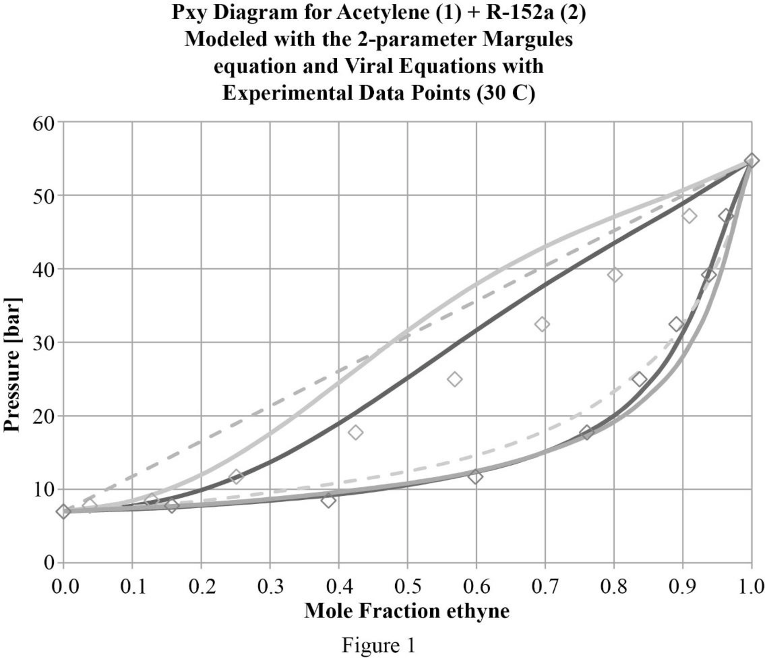
In figure (1) gamma phi approach is indicated by the dark solid line and the modified Raoult’s law is shown by the light solid line and the Raoult’s law by the dashed lines. There is a benefit for treating the system as a real gas instead of as an ideal gas. But at higher pressures, the correlation for bubble point is weaker which is because of the challenge in fitting Gibbs free energy into the model.