Given information: x=20 and 95% prediction interval
| x2513161929191630y4020333050373437 |
Formula Used:the formula to be usedwhen constructing a prediction interval for an individual response.
Let x* be a value of the explanatory variable x , let y∧=b0+b1x* be the predicted value corresponding to x* and let n be the sample size .A level 100(1−α)% prediction interval for an individual response is
y∧±tα/2.se1+1n+ ( x * − x ¯ )2∑ (x− x ¯ ) 2
Here, the critical value tα/2 is based on n−2 degrees of freedom.
se - Residual standard deviation =∑ (y− y ) 2 ∧ n−2
Test statistic t=(x1¯−x2¯)−(μ1−μ2) s 1 2 n 1 + s 2 2 n 2
Calculation:sample means and the sample variances can be calculated as shown.
xyx¯y¯x−x¯y−y¯ ( x− x ¯ )2 ( y− y ¯ )2254020.87535.1254.1254.87517.01562523.7656251320−7.875−15.12562.015625228.765631633−4.875−2.12523.7656254.5156251930−1.875−5.1253.51562526.26562529508.12514.87566.015625221.265631937−1.8751.8753.5156253.5156251634−4.875−1.12523.7656251.26562530379.1251.87583.2656253.515625
Sample means;
x¯=∑xnx¯=(35+13+16+19+29+19+16+30)8x¯=1678x¯=20.875
y¯=∑yny¯=(40+20+33+30+50+37+34+37)8y¯=2818y¯=35.125
Sample variances;
sx2=∑ (x− x ¯ ) 2 n−1sx2= (25−20.875)2+ (13−20.875)2+...........+ (30−20.875)28−1sx2=282.8757sx2=40.4107143sx=6.35694221
sy2=∑ (y− y ¯ ) 2 n−1sy2= (40−35.125)2+ (20−35.125)2+...........+ (37−35.125)28−1sy2=512.8757sy2=73.267857sy=8.5596645
The correlation coefficient is calculated as shown.
r=1(n−1)∑ (x− x ¯ )(y− y ¯ )sxsyr=1(8−1)(4.125)(4.875)+........+(9.125)(1.875)(6.35694221)(8.5596645)r=1(8−1)299.125(6.35694221)(8.5596645)r=0.785325
Also, the least square regression line can be calculated as shown.
y∧=b0+b1x
Here;
b1=rsysxb1=0.785325( 6.35694221 8.5596645)b1=1.0574
Here;
b0=y¯−b1x¯b0=35.125−(1.0574)(20.875)b0=13.051
Therefore,
y∧=b0+b1xy∧=13.051+1.0574x
Now we need to calculate the residuals to find the se - Residual standard deviation.
xyy∧=13.051+1.0574xy−y∧ ( y− y ∧ )2254039.4860.5140.264196132026.7972−6.797246.20193163329.96943.03069.184536193033.1416−3.14169.869651295043.71566.284439.49368193733.14163.858414.88725163429.96944.030616.24574303744.773−7.77360.41953
se= ∑ (y− y ) 2 ∧ n−2se= 0.264196+........+60.41953 8−2se= 196.56656se=32.76109se=5.72373
Finally we can now calculate the prediction interval for an individual response.
y∧±tα/2.se1+1n+ ( x * − x ¯ )2∑ (x− x ¯ ) 2
Here; when x=20 ;
y∧=13.051+1.057xy∧=13.051+1.057(20)y∧=34.199
And;
( x * − x ¯ ) 2 = (20−20.875) 2 =0.765625
And;
∑ (x− x ¯ )2=282.875
Therefore;
y∧±tα/2.se1+1n+ ( x * − x ¯ ) 2 ∑ (x− x ¯ ) 2 34.199±tα/2(5.72373)1+18+ 0.765625 282.87534.199±tα/2(5.72373)(1.0619353)34.199±tα/26.07823093467
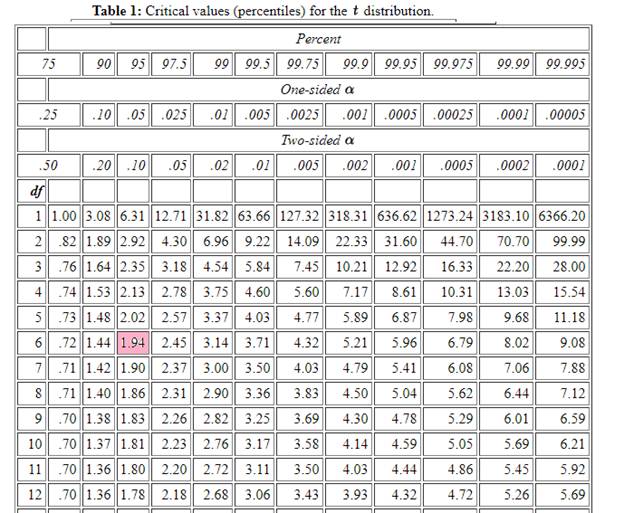
Please note there wasn’t a table given in the book to find corresponding t-value for the given confidence interval 95% and degrees of freedom 6 as shown below.
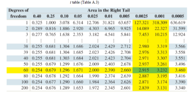
The t table below statescorresponding t-value for the given confidence interval 95% and degrees of freedom 6 can be read as 1.94 .


 Glencoe Algebra 1, Student Edition, 9780079039897...AlgebraISBN:9780079039897Author:CarterPublisher:McGraw Hill
 College Algebra (MindTap Course List)AlgebraISBN:9781305652231Author:R. David Gustafson, Jeff HughesPublisher:Cengage Learning
 Holt Mcdougal Larson Pre-algebra: Student Edition...AlgebraISBN:9780547587776Author:HOLT MCDOUGALPublisher:HOLT MCDOUGAL