
Concept explainers
Videos
a.
To find: The equation of the fitted least-squares line
a.
Explanation of Solution
Given:
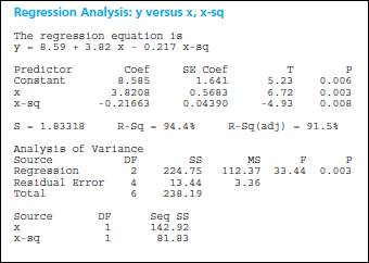
The Minitab output is:
Plot is:
From the provided output, the equation of the regression line is:
a.
To interpret: The value of
a.
Explanation of Solution
From the provided output, the coefficient of determination is 0.944. It means that 99.8% of the variation in the model is explained. Since, the value is large enough it means that the provided model is fit enough.
c.
To find: Whether the model is significant at 5% level of significance.
c.
Explanation of Solution
From the provided excel output; the p -value is equal to 0.000 which implies that the regression model is highly significant.
c.
To find: Whether there is sufficient evidence to show that the quadratic model provides a better fir to the data than a simple linear model.
c.
Explanation of Solution
The prediction equation relating
d.
To find: The number of defective items produced for an operator whose average output per hour is 25 and whose machine was serviced 3 weeks ago.
d.
Explanation of Solution
Since, the p -value is less than the level of significance. Thus, it could be said that the quadratic model provided a better fit than a simple linear model
e.
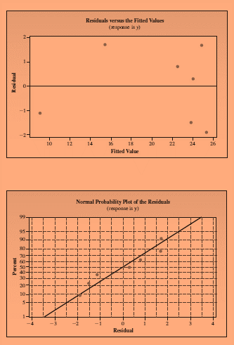
To explain: Whether normality assumptions have been violated using the residual plot.
e.
Explanation of Solution
From the provided residual plot, it could be said that there is no violation of normality assumptions. It means that model is well fitted.
Want to see more full solutions like this?
Chapter 13 Solutions
EBK INTRODUCTION TO PROBABILITY AND STA


- Population Genetics In the study of population genetics, an important measure of inbreeding is the proportion of homozygous genotypesthat is, instances in which the two alleles carried at a particular site on an individuals chromosomes are both the same. For population in which blood-related individual mate, them is a higher than expected frequency of homozygous individuals. Examples of such populations include endangered or rare species, selectively bred breeds, and isolated populations. in general. the frequency of homozygous children from mating of blood-related parents is greater than that for children from unrelated parents Measured over a large number of generations, the proportion of heterozygous genotypesthat is, nonhomozygous genotypeschanges by a constant factor 1 from generation to generation. The factor 1 is a number between 0 and 1. If 1=0.75, for example then the proportion of heterozygous individuals in the population decreases by 25 in each generation In this case, after 10 generations, the proportion of heterozygous individuals in the population decreases by 94.37, since 0.7510=0.0563, or 5.63. In other words, 94.37 of the population is homozygous. For specific types of matings, the proportion of heterozygous genotypes can be related to that of previous generations and is found from an equation. For mating between siblings 1 can be determined as the largest value of for which 2=12+14. This equation comes from carefully accounting for the genotypes for the present generation the 2 term in terms of those previous two generations represented by for the parents generation and by the constant term of the grandparents generation. a Find both solutions to the quadratic equation above and identify which is 1 use a horizontal span of 1 to 1 in this exercise and the following exercise. b After 5 generations, what proportion of the population will be homozygous? c After 20 generations, what proportion of the population will be homozygous?arrow_forwardUrban Travel Times Population of cities and driving times are related, as shown in the accompanying table, which shows the 1960 population N, in thousands, for several cities, together with the average time T, in minutes, sent by residents driving to work. City Population N Driving time T Los Angeles 6489 16.8 Pittsburgh 1804 12.6 Washington 1808 14.3 Hutchinson 38 6.1 Nashville 347 10.8 Tallahassee 48 7.3 An analysis of these data, along with data from 17 other cities in the United States and Canada, led to a power model of average driving time as a function of population. a Construct a power model of driving time in minutes as a function of population measured in thousands b Is average driving time in Pittsburgh more or less than would be expected from its population? c If you wish to move to a smaller city to reduce your average driving time to work by 25, how much smaller should the city be?arrow_forward

 Functions and Change: A Modeling Approach to Coll...AlgebraISBN:9781337111348Author:Bruce Crauder, Benny Evans, Alan NoellPublisher:Cengage Learning
 Linear Algebra: A Modern IntroductionAlgebraISBN:9781285463247Author:David PoolePublisher:Cengage Learning
 Algebra & Trigonometry with Analytic GeometryAlgebraISBN:9781133382119Author:SwokowskiPublisher:Cengage