STATISTICS FOR ENGINEERS+SCI.-ACCESS
4th Edition
ISBN: 9781259998584
Author: Navidi
Publisher: MCG
expand_more
expand_more
format_list_bulleted
Videos
Textbook Question
Chapter 1.3, Problem 5E
A certain reaction was run several times using each of two catalysts, A and B. The catalysts were supposed to control the yield of an undesirable side product. Results, in units of percentage yield, for 24 runs of catalyst A and 20 runs of catalyst B are as follows:
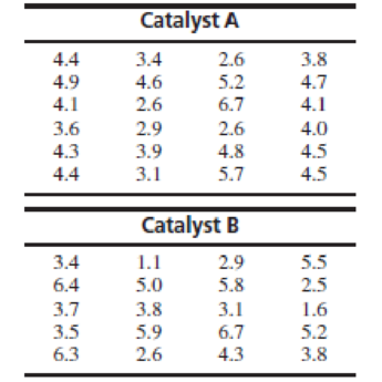
- a. Construct a histogram for the yields of each catalyst.
- b. Construct comparative boxplots for the yields of the two catalysts.
- c. Using the boxplots, what differences can be seen between the results of the yields of the two catalysts?
Expert Solution & Answer
Want to see the full answer?
Check out a sample textbook solution
Students have asked these similar questions
Three types of medium sized cars assembled in New Zealand have been test driven by a motoring magazine and compared on a variety of criteria. In the area of fuel efficiency performance, five cars of each brand were each test driven 1000 km; the km per litre data are obtained as follows (kilometres per litre): Brand A (7.6; 8.4; 8.0; 7.6; 8.4). Brand B (7.8; 8.0; 9.1; 8.5; 9.6). Brand C (9.6; 10.4; 9.2; 9.7; 10.6). SSE = 4.26 and TSS = 13.693. what is the critical value at 5% significance level
Three types of medium sized cars assembled in New Zealand have been test driven by a motoring magazine and compared on a variety of criteria. In the area of fuel efficiency performance, five cars of each brand were each test driven 1000 km; the km per litre data are obtained as follows (kilometres per litre): Brand A (7.6; 8.4; 8.0; 7.6; 8.4). Brand B (7.8; 8.0; 9.1; 8.5; 9.6). Brand C (9.6; 10.4; 9.2; 9.7; 10.6). SSE = 4.26 and TSS = 13.693. What is the value of the F-statistic (rounded off 2 decimals)?
The owner of a new car conducts a series of six gas mileage tests and obtains the following results, expressed in miles per gallon: 3., 22.7, 21.4, 20.6, and 21.4. 20.9. Find the mode for these data.
Chapter 1 Solutions
STATISTICS FOR ENGINEERS+SCI.-ACCESS
Ch. 1.1 - Each of the following processes involves sampling...Ch. 1.1 - If you wanted to estimate the mean height of all...Ch. 1.1 - True or false: a. A simple random sample is...Ch. 1.1 - A sample of 100 college students is selected from...Ch. 1.1 - A certain process for manufacturing integrated...Ch. 1.1 - Refer to Exercise 5. True or false: a. If the...Ch. 1.1 - To determine whether a sample should be treated as...Ch. 1.1 - A medical researcher wants to determine whether...Ch. 1.1 - A medical researcher wants to determine whether...Ch. 1.2 - True or false: For any list of numbers, half of...
Ch. 1.2 - Is the sample mean always the most frequently...Ch. 1.2 - Is the sample mean always equal to one of the...Ch. 1.2 - Is the sample median always equal to one of the...Ch. 1.2 - Find a sample size for which the median will...Ch. 1.2 - For a list of positive numbers, is it possible for...Ch. 1.2 - Is it possible for the standard deviation of a...Ch. 1.2 - In a certain company, every worker received a...Ch. 1.2 - In another company, every worker received a 5%...Ch. 1.2 - A sample of 100 adult women was taken, and each...Ch. 1.2 - In a sample of 20 men, the mean height was 178 cm....Ch. 1.2 - Each of 16 students measured the circumference of...Ch. 1.2 - Refer to Exercise 12. a. If the measurements for...Ch. 1.2 - There are 10 employees in a particular division of...Ch. 1.2 - Quartiles divide a sample into four nearly equal...Ch. 1.2 - In each of the following data sets, tell whether...Ch. 1.3 - The weather in Los Angeles is dry most of the...Ch. 1.3 - Forty-five specimens of a certain type of powder...Ch. 1.3 - Refer to Table 1.2 (in Section 1.2). Construct a...Ch. 1.3 - Following are measurements of soil concentrations...Ch. 1.3 - A certain reaction was run several times using...Ch. 1.3 - Sketch a histogram for which a. The mean is...Ch. 1.3 - The figure below is a histogram showing the...Ch. 1.3 - The histogram below presents the compressive...Ch. 1.3 - Refer to Table 1.4 (in Section 1.3). a. Using the...Ch. 1.3 - Refer to Table 1.5 (in Section 1.3). a. Using the...Ch. 1.3 - The following table presents the number of...Ch. 1.3 - Which of the following statistics cannot be...Ch. 1.3 - A sample of 100 resistors has an average...Ch. 1.3 - Following are boxplots comparing the amount of...Ch. 1.3 - Following are summary statistics for two data...Ch. 1.3 - Match each histogram to the box plot that...Ch. 1.3 - Prob. 17ECh. 1.3 - Match each scatterplot to the statement that best...Ch. 1.3 - Prob. 19ECh. 1 - A vendor converts the weights on the packages she...Ch. 1 - Refer to Exercise 1. The vendor begins using...Ch. 1 - The specification for the pull strength of a wire...Ch. 1 - A coin is tossed twice and comes up heads both...Ch. 1 - The smallest number on a list is changed from 12.9...Ch. 1 - There are 15 numbers on a list, and the smallest...Ch. 1 - There are 15 numbers on a list, and the mean is...Ch. 1 - The article The Selection of Yeast Strains for the...Ch. 1 - Concerning the data represented in the following...Ch. 1 - True or false: In any boxplot, a. The length of...Ch. 1 - For each of the following histograms, determine...Ch. 1 - In the article Occurrence and Distribution of...Ch. 1 - The article Vehicle-Arrival Characteristics at...Ch. 1 - The cumulative frequency and the cumulative...Ch. 1 - The article Hydrogeochemical Characteristics of...Ch. 1 - Water scarcity has traditionally been a major...Ch. 1 - Prob. 18SECh. 1 - The article The Ball-on-Three-Ball Test for...
Knowledge Booster


Learn more about
Need a deep-dive on the concept behind this application? Look no further. Learn more about this topic, statistics and related others by exploring similar questions and additional content below.Similar questions
- Urban Travel Times Population of cities and driving times are related, as shown in the accompanying table, which shows the 1960 population N, in thousands, for several cities, together with the average time T, in minutes, sent by residents driving to work. City Population N Driving time T Los Angeles 6489 16.8 Pittsburgh 1804 12.6 Washington 1808 14.3 Hutchinson 38 6.1 Nashville 347 10.8 Tallahassee 48 7.3 An analysis of these data, along with data from 17 other cities in the United States and Canada, led to a power model of average driving time as a function of population. a Construct a power model of driving time in minutes as a function of population measured in thousands b Is average driving time in Pittsburgh more or less than would be expected from its population? c If you wish to move to a smaller city to reduce your average driving time to work by 25, how much smaller should the city be?arrow_forwardThe Senator of Azenator State, is worried about the rising numbers in high blood pressure related deaths in his Jurisdiction and wants an end to this canker. A reputable medical research officer has claimed that, the situation is probably as a result of the ageing population of his State. The blood pressures, Y (mmHg), and Ages, X (years) of 10 hospital patients were sampled from Azenator State and summarized below. Patient A B C D E F G H I J Age(X) in Years 20 25 50 30 45 60 10 15 35 70 BP(Y) in (mmHg) 80 85 125 90 100 135 80 70 100 140 NB: Approximate to 2 decimal placesUse the table to answer the questions that follow;i) Calculate the product moment correlation coefficient for the data and interpret your result.ii) If the Senator decides to purchase and distribute Norvasc (a medicine that reduces blood pressure), based on your results in (i), which age group (youth or old adults) should be given priority? Briefly explain your answer. iii) Give a reason to support fitting…arrow_forwardConsider a cohort study to compare the mortality rate of myocardial infarction (MI) in men with sedentary work (exposed group) to men with physically active work (unexposed). If in the exposed, there were 36,000 person (man) years of observation and 126 deaths whereas the unexposed had 24,000 man-years of observation and 44 deaths. Compute the following a) Mortality rate in each cohort? b) What is the relative risk of dying, comparing these 2 groups? c) What is the attributable risk of sedentary work? d) What is the attributable benefit of physical activity? e) If we assume that MI is associated with the mortality in this cohort (causality), what proportion of the disease in the higher group is potentially preventable?arrow_forward
- Penicillin is produced by the Penicillin fungus, which is grown in a broth whose sugar content must be carefully controlled. Several samples of broth were taken on three successive days, and the amount of dissolved sugars, in milligrams per milliliter, was measured on each sample. The results were as follows. Day 1 : 4.9 5.4 5.3 4.9 5.2 5.1 5.4 4.9 5.1 5.1 4.9 5.4 Day 2 : 5.5 5.2 5.1 5.0 5.3 5.4 5.3 5.2 5.4 5.3 5.4 5.1 Day 3 : 5.8 5.0 5.4 5.5 5.5 5.5 4.8 5.5 5.2 4.9 5.5 5.0 Construct an ANOVA table. Round your answers to four decimal places as needed. One-way ANOVA: Sugar Concentration Source DF SS MS F P Days Error Total Is there enough evidence to conclude that the mean sugar concentration…arrow_forwardA research group is interested in the relationship between exposure to mold in households after a major hurricane and the onset of acute respiratory illness in children. Suppose an observational study is conducted over 10 years following the natural disaster and the following two-by-two table was created in order to address the relationship between exposure and outcome. Acute Respiratory Illness No Acute Respiratory Illness Total Mold 378 156 534 No Mold 73 260 333 Total 451 416 867 Calculate the incidence of acute respiratory illness in the exposed and unexposed. Calculate the relative risk for ARI due to exposure in this study Interpret your findings from part Barrow_forwardAn insurance company selected samples of clients under 18 years of age and over 18 and recorded the number of accidents they had in the previous year. The results are shown below. Under Age 18 Over Age 18 n1 = 500 n2 = 600 Number of accidents = 180 Number of accidents = 150 We are interested in determining if the accident proportions differ between the two age groups.arrow_forward
- Periodically, the county Water Department tests the drinking water of homeowners for contaminants such as lead and copper. The lead and copper levels in water specimens collected in 1998 for a sample of 10 residents of a subdevelopement of the county are shown below. lead (μμg/L) copper (mg/L) 4.44.4 0.6430.643 2.42.4 0.570.57 1.51.5 0.460.46 2.62.6 0.8950.895 5.95.9 0.20.2 3.43.4 0.540.54 3.83.8 0.2450.245 1.61.6 0.5830.583 5.75.7 0.7690.769 1.71.7 0.2150.215 (a) Construct a 9999% confidence interval for the mean lead level in water specimans of the subdevelopment. ≤μ≤≤μ≤ (b) Construct a 9999% confidence interval for the mean copper level in water specimans of the subdevelopment. ≤μ≤≤μ≤arrow_forwardFifteen adult males between the ages of 35 and 50 participated in a study to evaluate the effect of diet and exercise on blood cholesterol levels. The total cholesterol was measured in each subject initially and then three months after participating in an aerobic exercise program and switching to a low-fat diet. The data are shown in the following table.arrow_forwardA researcher wishes to study the relationship between education and income separately for individuals who have college degrees, and for those who don't. To this end, he interviews 100 individuals in each category. Survey results are listed in the table below. non college graduates college graduates avg education 13 yr 18 yr std. dev. education 2 yr 1.2 yr Sxx 396 yr2 143 yr2 Avg. Income $67,200 $84,950 std. dev. income $9,400 $10,500 correlation coefficient .25 .15 a. Use the data above to find point estimates for regression coefficients B0NG and B1NG for non-college graduates and BoG and B1G for college graduates. b. Propose an unbiased estimator for the difference theta=B1G - B1NG in slope coefficients for the two sub-populations, and show that B(theta hat)= 0. c. Assume that the error terms ENG and EG for non-graduates and graduates, respectively, are both distributed normally, with known standard deviation oENG = oEG = $ 10,000. In that case, determine the…arrow_forward
- A study was undertaken to determine whether there was a significant weight (in lb) loss after one year course of therapy for diabetes, and whether the amount of weight (in lb) loss was related to initial weight. The following table gives the initial weight (x) and weight after one year of therapy (y) for 16 newly diagnosed adult diabetic patients.arrow_forwardAn automotive engineer is investigating two different types of metering devices for an electronic fuel injection system to determine whether they differ in their fuel mileage performance. The system is installed on 10 different cars, and a test is run with each metering device on each car. The data is provided below: Metering Device Car 1 2 1 17.6 16.8 2 19.4 20.0 3 18.2 17.6 4 17.1 16.4 5 15.3 16.0 6 15.9 15.9 7 16.3 16.5 8 18.0 18.4 9 17.3 16.4 10 19.1 20.1 Is there a significant difference between the means of the two metering devices? Use . Interpret the result in the context of the problem. An article in the journal Hazardous Waste and Hazardous Materials (Vol. 6, 1989) reported the results of an analysis of the weight of calcium in standard cement and cement doped with lead. Reduced levels of calcium would indicate that the hydration mechanism in the cement is blocked…arrow_forwardFollowing some school examinations, Ajok is studying the results of the 16 students in her class. The mark for paper 1, , and the mark for paper 2, , for each student are summarised in the following statistics. X Mean= 35.75 , Y Mean=25.75 , St Dev of X=8.05 ,St Dev of Y=12.3 , R=0.75 Ajok decides to examine these data in more detail and plots the marks for each of the 16 students on the scatter diagram. Graph Attached Using the summary statistics above, calculate the equation of the line of regression of y on x for these 16 students, giving your answer in the form yhat = a+bx Ajok decides to omit the data point (38,0) and examine the other 15 students’ marks. The correlation coefficient is now R = 0.95. Explain why you think Ajok decides to omit the data point (38.0). Using the following summary statistics calculate the equation of the line of regression of y on x for these 15 students X Mean= 35.6 , Y Mean=27.47 , St Dev of X=8.31 ,St Dev of Y=10.56, R=0.95 Give your answer…arrow_forward
arrow_back_ios
SEE MORE QUESTIONS
arrow_forward_ios
Recommended textbooks for you
 Functions and Change: A Modeling Approach to Coll...AlgebraISBN:9781337111348Author:Bruce Crauder, Benny Evans, Alan NoellPublisher:Cengage Learning
 Glencoe Algebra 1, Student Edition, 9780079039897...AlgebraISBN:9780079039897Author:CarterPublisher:McGraw Hill
Functions and Change: A Modeling Approach to Coll...
Algebra
ISBN:9781337111348
Author:Bruce Crauder, Benny Evans, Alan Noell
Publisher:Cengage Learning
Glencoe Algebra 1, Student Edition, 9780079039897...
Algebra
ISBN:9780079039897
Author:Carter
Publisher:McGraw Hill
Hypothesis Testing using Confidence Interval Approach; Author: BUM2413 Applied Statistics UMP;https://www.youtube.com/watch?v=Hq1l3e9pLyY;License: Standard YouTube License, CC-BY
Hypothesis Testing - Difference of Two Means - Student's -Distribution & Normal Distribution; Author: The Organic Chemistry Tutor;https://www.youtube.com/watch?v=UcZwyzwWU7o;License: Standard Youtube License