Concept explainers
Videos
House prices This chapter has considered many aspects of
- a. Construct a
scatterplot matrix. Identify the plots that pertain to selling price as a response variable. Interpret and explain how the highly discrete nature of x2 and x3 affects the plots. - b. Fit the model. Write down the prediction equation and interpret the coefficient of size of home by its effect when x2 and x3 are fixed.
- c. Show how to calculate R2 from SS values in the ANOVA table. Interpret its value in the context of these variables.
- d. Find and interpret the
multiple correlation . - e. Show all steps of the F test that selling price is independent of these predictors. Explain how to obtain the F statistic from the mean squares in the ANOVA table.
- f. Report the t statistic for testing H0: β2 = 0. Report the P-value for Ha: β2 < 0 and interpret. Why do you think this effect is not significant? Does this imply that the number of bedrooms is not associated with selling price?
- g. Construct and examine the histogram of the residuals for the multiple regression model. What does this describe, and what does it suggest?
- h. Construct and examine the plot of the residuals plotted against size of home. What does this describe, and what does it suggest?
a.
Draw a scatterplot matrix.
Identify the plots that identify selling price as a response variable.
Interpret and explain the manner in which the highly discrete nature of
Answer to Problem 60CP
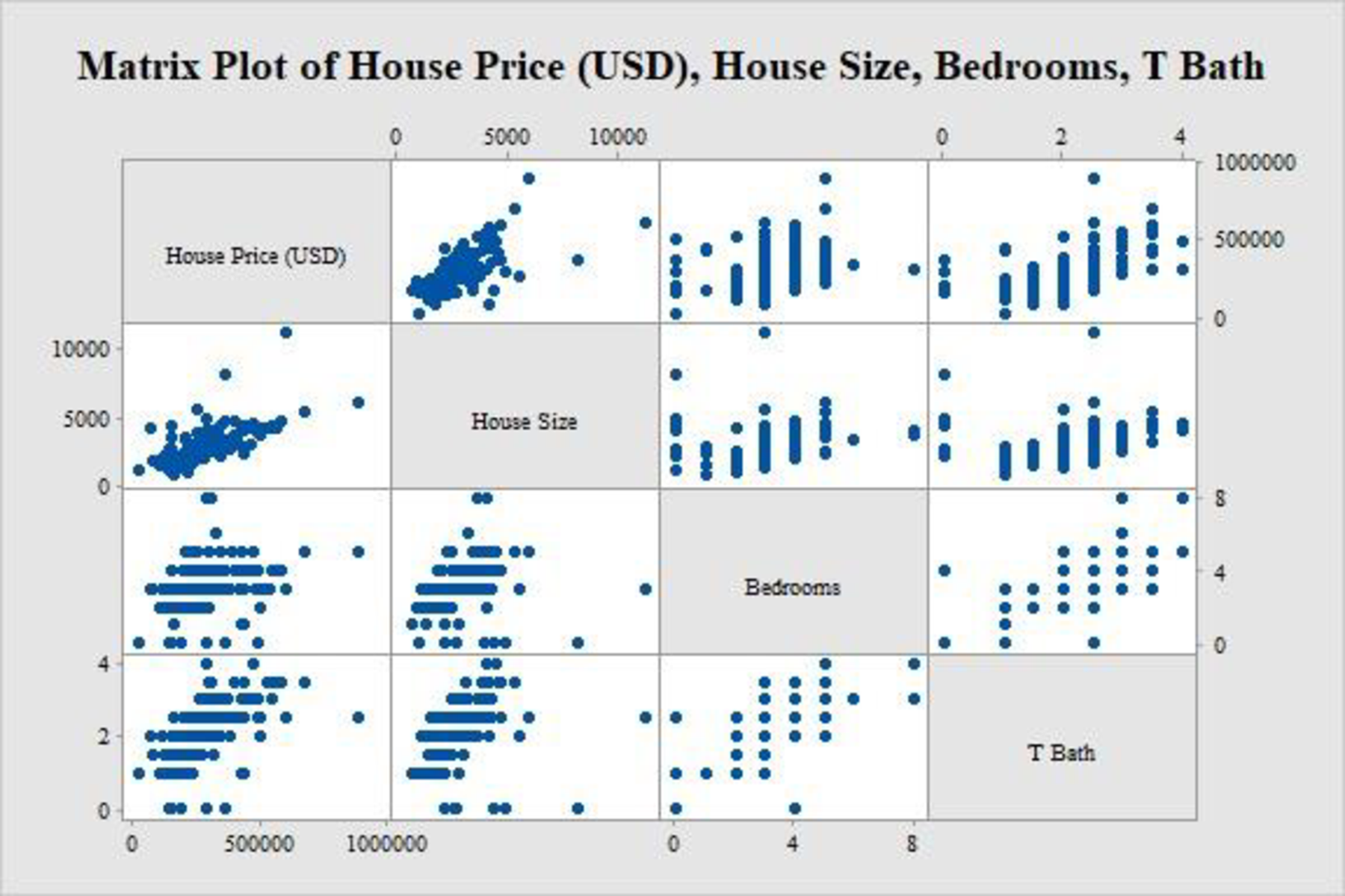
The scatterplot matrix is as follows:
Explanation of Solution
Calculation:
The data relate the selling price of home to the size of the home, the number of bedrooms, and the number of bathrooms.
Denote the response variable and selling price of home as y, the predictor and size of home as
Scatterplot matrix:
Software procedure:
Step by step procedure to draw the scatterplot matrix using the MINITAB software:
- Choose Graph > Matrix Plots > Simple > OK.
- Enter the columns of House Price (USD), House Size, Bedrooms, and T Bath under Graph variables.
- Click OK in all dialogue boxes.
Thus, the scatterplot matrix is obtained.
Interpretation:
The plots in the top row of the scatterplot matrix have the house prices along the vertical axis and the other variables in the corresponding horizontal axes. Now, it is customary to plot the response variable along the vertical axis and the predictor variable along the horizontal axis.
Thus, the plots across the top row pertain to selling price as a response variable.
The number of bedrooms and the number of bathrooms are highly discrete, which can only take limited number of values. Each of these discrete values has many observations and it is reflected in the above graph. Since these variables are discrete, the regression or prediction procedure for continuous predictors may not be well-defined.
b.
Fit a model and give the prediction equation.
Interpret the effect of coefficient of size of home when
Answer to Problem 60CP
The prediction equation is as follows:
Explanation of Solution
Calculation:
Regression equation:
Software procedure:
Step by step procedure to obtain the regression equation using the MINITAB software:
- Choose Stat > Regression > Regression > Fit Regression Model.
- Enter the column of y under House Price(USD).
- Enter the columns of House size, Bedrooms, and T Bath under Continuous predictors.
- Choose Results and select Analysis of variance, Model summary, Coefficients, Regression Equation.
- Click OK in all dialogue boxes.
Output obtained using MINITAB is given below:
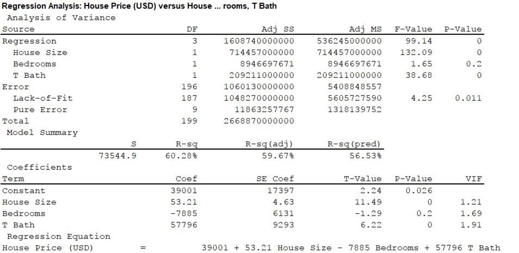
From Regression equation is MINTAB output and the prediction equation is as follows:
Significance of the slope:
In a multiple regression equation, the slope corresponding to a particular explanatory variable signifies the effect of that explanatory variable on the response variable while keeping the other explanatory variables at a fixed level. The slope gives the amount of change in the response variable for unit increase in the explanatory variable. A positive slope implies that the response variable increases when the explanatory variable increases, whereas a negative slope implies that the response variable decreases when the explanatory variable increases.
From the MINITAB output, the slope corresponding to House size is 53.21, which is positive.
It is clear that a unit increase in the House size increases the selling price of a house by $53.21 using the explanation regarding the significance of slope.
c.
Explain the procedure to calculate
Answer to Problem 60CP
The value of
Explanation of Solution
Calculation:
The statistic
The statistic
The numerator gives the regression sum of squares, which is
From Part b., the column “Adj SS” of the “Analysis of Variance” section provides the sum of squares for the test. The sum of square (SS) value is 1,608,740,000,000 corresponding to the Source “Regression” and the SS value is 2,668,870,000,000 corresponding to “Total”.
The value of
Thus, the value of
Interpretation:
In this case, the value of
d.
Calculate and interpret the multiple correlation.
Answer to Problem 60CP
The multiple correlation is 0.78.
Explanation of Solution
Calculation:
It is known that
From Part c., the value of
Thus, the multiple correlation, R is the positive square root of
Thus, the multiple correlation is 0.78.
Interpretation:
The multiple correlation coefficient is the correlation coefficient between the observed response variable, y and the predicted value of the response variable,
The value of multiple correlation is 0.78, which is quite close to 1. Thus, there is quite strong relationship between the observed selling prices and selling prices using the given prediction model.
e.
Show all steps of the F test for predicting the selling price.
Explain the procedure to obtain the F statistic from mean squares in the ANOVA table.
Explanation of Solution
Calculation:
Step 1: Assumptions:
The multiple regression holds for the selling price of houses. There is a normal distribution for y with the same standard deviation at each combination of values of the predictors in the model. The data is collected randomly.
Step 2: Hypotheses:
Assume that
Null hypothesis:
That is, house-selling price does not depend on size of home, number of bedrooms, and number of bathrooms.
Alternative hypothesis:
That is, house-selling price depends on size of home, number of bedrooms, and number of bathrooms.
Step 3: Test statistic:
The formula for F test statistic is as follows:
From Part b., the column “F-value” of the “Analysis of Variance” section provides the F-test statistic values. Corresponding to the Source “Regression”, The F-value is 99.14.
Thus, F-test statistic is 99.14.
Step 4: P-value:
From Part b., the column “P-value” of the “Analysis of Variance” section provides the P-values for the test. Corresponding to the Source “Regression”, the P-value is 0.
Step 5: Conclusion:
Decision rule:
If
Here, P-value is less than the most commonly used levels of significance like 0.05, 0.01, and 0.10.
Therefore, reject the null hypothesis.
Thus, there is strong evidence that at least one of House size, number of bedrooms, and number of bathrooms is useful for predicting the House price.
f.
Find the t test statistic for the given hypotheses.
Find the P-value for the given alternative hypothesis.
Explain the reason that the effect of number of bedrooms is not significant.
Check whether it is implied that the number of bedrooms is not associated with the selling price of the house.
Answer to Problem 60CP
The value of t-test statistic is –1.29.
The P-value is 0.1.
Explanation of Solution
Calculation:
It is assumed that
The given hypotheses are as follows:
Null hypothesis:
That is, the selling price of house does not depend on the number of bedrooms.
Alternative hypothesis:
That is, house selling price decreases with the number of bedrooms.
The formula for t-test statistic is as follows:
Here “
From Part b., the column “T-value” of the “Coefficients” section provides the T-test statistic values. The T-value corresponding to “Bedrooms” is –1.29.
Thus, the value of t-test statistic is –1.29.
P-value:
From Part b., the P-value is 0.2
The P-value for two-tailed test with critical value
The P-value for left-tailed test with critical value
Hence, for the left-tailed test, the P-value is calculated from the P-value of the two-tailed test as follows:
Thus, P-value is 0.1.
Decision rule:
If
Here, P-value is greater than the most commonly used levels of significance like 0.05, 0.01.
Therefore, fail to reject the null hypothesis.
Thus, there is no evidence that the selling price of house depends on the number of bedrooms at levels of significance 0.05 and 0.01.
Here, P-value is equal with the level of significance 0.10.
Therefore, reject the null hypothesis.
Thus, there is enough evidence that the selling price of house depends on the number of bedrooms at level of significance 0.10.
The effect of number of bedrooms is not significant on house price because the other explanatory variables have an effect on the house selling price. If it is used independently, the effect may be significant.
Thus, it cannot be said that the number of bedrooms is not associated with the selling price.
g.
Draw the histogram of the residuals and examine it.
State the conclusions from the graph.
Answer to Problem 60CP
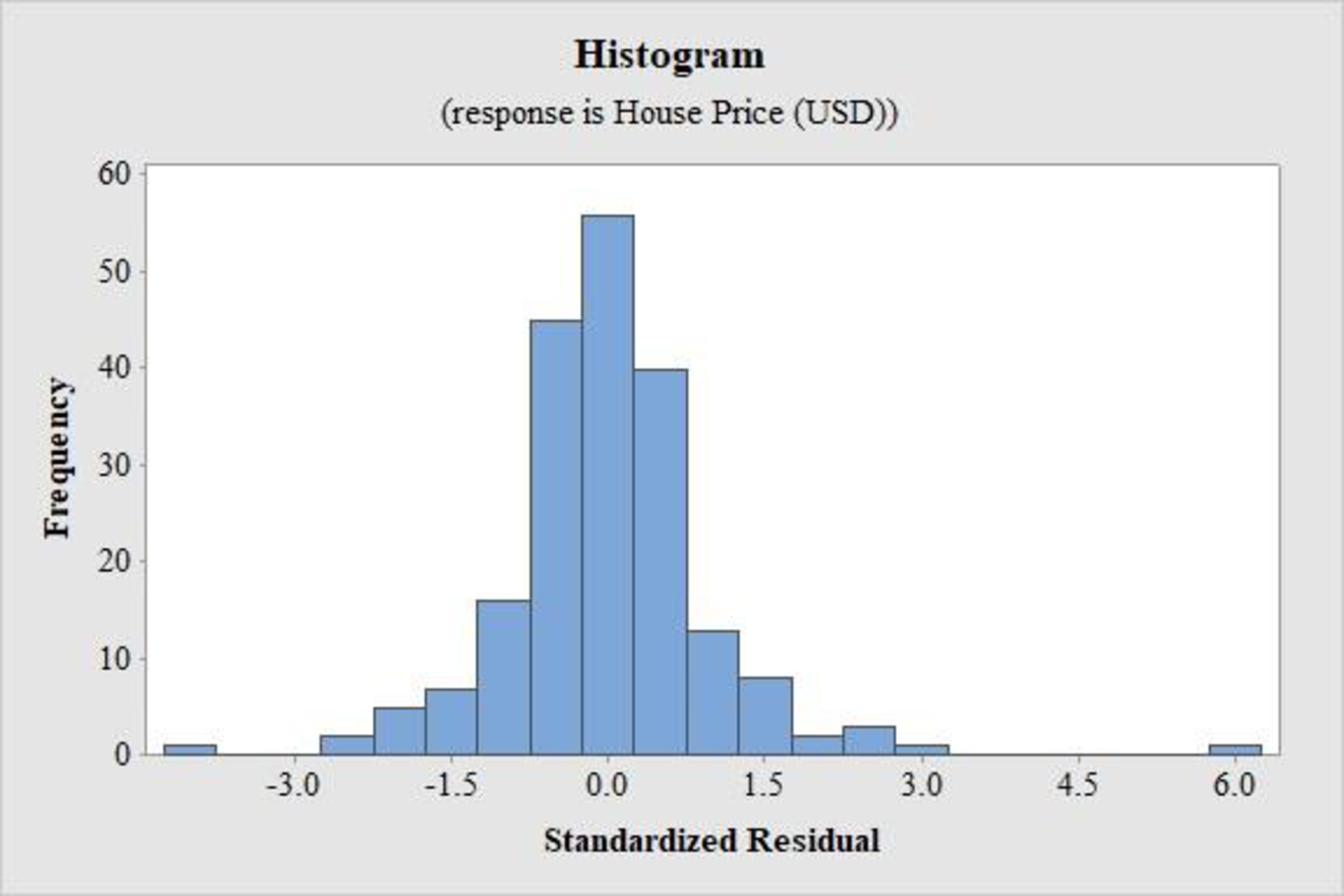
The histogram for the residuals is as follows:
Explanation of Solution
Calculation:
Histogram of standardized residuals:
Software procedure:
Step by step procedure to obtain the histogram of the standardized residuals using the MINITAB software:
- Choose Stat > Regression > Regression > Fit Regression Model.
- Enter the column of y under House Price(USD).
- Enter the columns of House size, Bedrooms, and T Bath under Continuous predictors.
- Choose Results and select Analysis of variance, Model summary, Coefficients, Regression Equation.
- Choose Graphs.
- Choose Standardized under Residuals for plots and select Histogram for residuals.
- Click OK in all dialogue boxes.
Thus, the histogram of the residuals is obtained.
Interpretation:
The histogram of the standardized residuals in this case is approximately bell-shaped. However, there is one outlier to the left and one extreme outlier to the right.
Thus, the graph indicates that the distribution of the conditional distribution of y at given values of the explanatory variables is approximately normal.
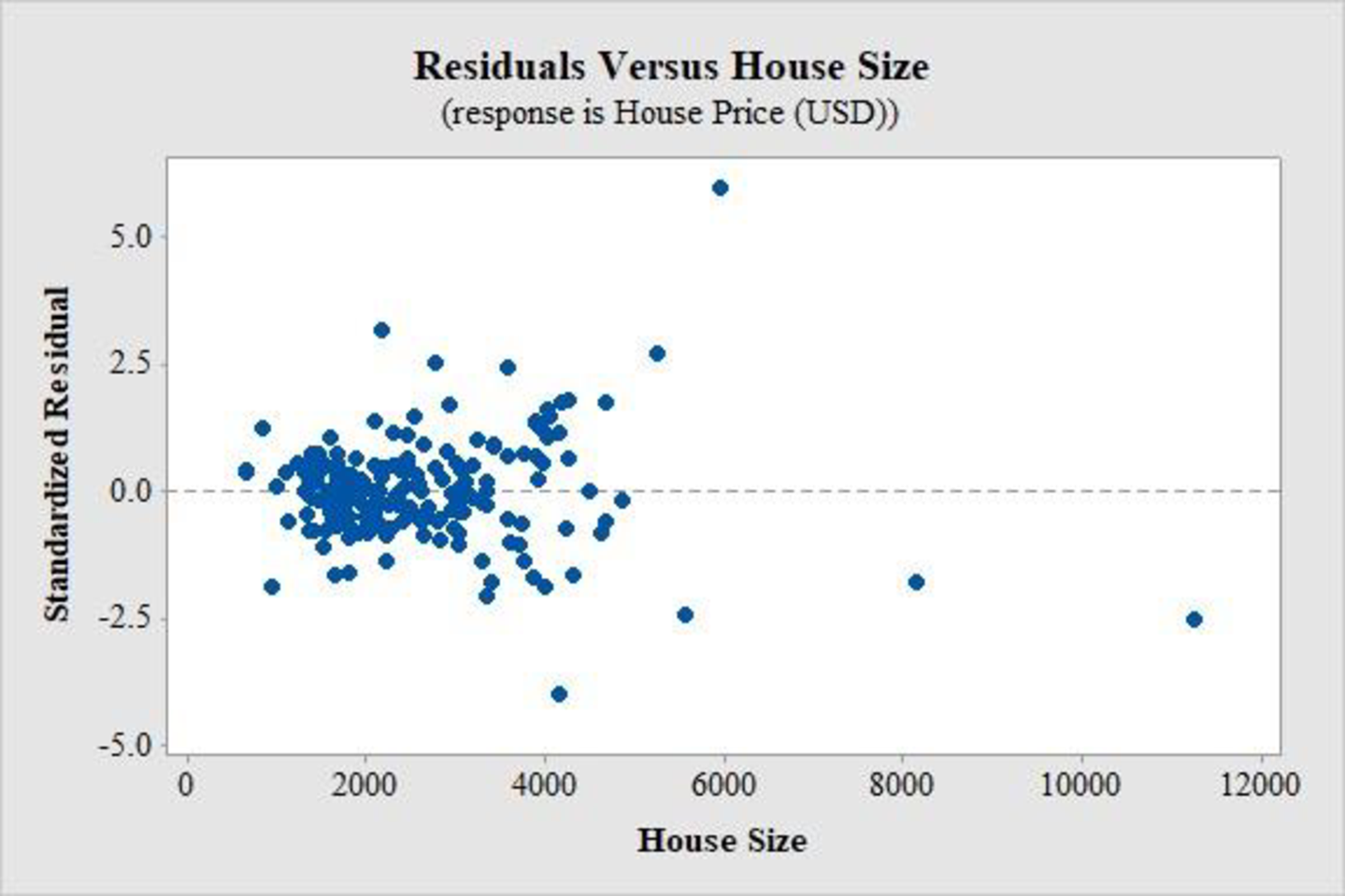
h.
Draw the plot of the residuals against size of home and examine it.
State the conclusions from the graph.
Answer to Problem 60CP
The plot for the residuals is as follows:
Explanation of Solution
Calculation:
Plot of residuals against size of home:
Software procedure:
Step by step procedure to obtain the histogram of the standardized residuals using the MINITAB software:
- Choose Stat > Regression > Regression > Fit Regression Model.
- Enter the column of y under House Price(USD).
- Enter the columns of House size, Bedrooms, and T Bath under Continuous predictors.
- Choose Results and select Analysis of variance, Model summary, Coefficients, Regression Equation.
- Choose Graphs.
- Choose Standardized under Residuals for plots.
- Under Residuals versus the variable, enter the column of House Size.
- Click OK in all dialogue boxes.
Thus, the plot of the residuals is obtained.
Interpretation:
The plot of the standardized residuals in this case is quite well-scattered and does not show any specific pattern. However, there is one value of the standardized residuals that is extremely high as compared to the others and one value that is fairly low. Moreover, the plot seems to become more scattered with an increase in house sizes.
Thus, the plot of residuals indicates that the relationship between the selling price and house sizes is quite straight, although a slightly greater deviation from the linearity occurs when house size increases.
Want to see more full solutions like this?
Chapter 13 Solutions
Statistics, Books a la Carte Edition Plus MyLab Statistics with Pearson eText -- Access Card Package (4th Edition)
Additional Math Textbook Solutions
Introductory Statistics
Fundamentals of Statistics (5th Edition)
Elementary Statistics (13th Edition)
Basic Business Statistics, Student Value Edition (13th Edition)
Elementary Statistics: Picturing the World (6th Edition)


 Elementary Linear Algebra (MindTap Course List)AlgebraISBN:9781305658004Author:Ron LarsonPublisher:Cengage Learning
 Glencoe Algebra 1, Student Edition, 9780079039897...AlgebraISBN:9780079039897Author:CarterPublisher:McGraw Hill
 Big Ideas Math A Bridge To Success Algebra 1: Stu...AlgebraISBN:9781680331141Author:HOUGHTON MIFFLIN HARCOURTPublisher:Houghton Mifflin Harcourt