
Videos
a.
To find:The value of
a.
Answer to Problem 16E
The value of
Explanation of Solution
Given information: The data is shown below.
| x | 12 | 17 | 3 | 17 | 16 | 11 | 14 | 9 |
| y | 13 | 14 | 16 | 13 | 14 | 14 | 13 | 14 |
Calculation:
The MINITAB is shown below,
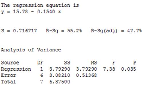
Figure-1
From Figure-1 it is clear that the value of
b.
To find: The value of
b.
Answer to Problem 16E
The value of
Explanation of Solution
Given information: The data is shown below.
| x | 12 | 17 | 3 | 17 | 16 | 11 | 14 | 9 |
| y | 13 | 14 | 16 | 13 | 14 | 14 | 13 | 14 |
Calculation:
From Figure-1 it is clear that the value of
c.
To find: The value of squares for
c.
Answer to Problem 16E
The value of squares for
Explanation of Solution
Given information: The data is shown below.
| x | 12 | 17 | 3 | 17 | 16 | 11 | 14 | 9 |
| y | 13 | 14 | 16 | 13 | 14 | 14 | 13 | 14 |
Calculation:
The table is shown below.
| 12 | -0.38 | 0.1444 |
| 17 | 4.62 | 21.3444 |
| 3 | -9.38 | 87.9844 |
| 17 | 4.62 | 21.3444 |
| 16 | 3.62 | 13.1044 |
| 11 | -1.38 | 1.9044 |
| 14 | 1.62 | 2.6244 |
| 9 | -3.38 | 11.4244 |
Thus, the value of squares for
d.
To find:The value of standard error of
d.
Answer to Problem 16E
The value of standard error of
Explanation of Solution
Given information: The data is shown below.
| x | 12 | 17 | 3 | 17 | 16 | 11 | 14 | 9 |
| y | 13 | 14 | 16 | 13 | 14 | 14 | 13 | 14 |
Calculation:
The value of
Thus, the value of standard error of
e.
To find:The critical value.
e.
Answer to Problem 16E
The critical value is
Explanation of Solution
Given information: The data is shown below.
| x | 12 | 17 | 3 | 17 | 16 | 11 | 14 | 9 |
| y | 13 | 14 | 16 | 13 | 14 | 14 | 13 | 14 |
Calculation:
The degree of freedom is,
The critical value is
f.
To find:The margin of error.
f.
Answer to Problem 16E
The margin of error is
Explanation of Solution
Given information: The data is shown below.
| x | 12 | 17 | 3 | 17 | 16 | 11 | 14 | 9 |
| y | 13 | 14 | 16 | 13 | 14 | 14 | 13 | 14 |
Calculation:
The margin of error is,
Thus, the margin of error is
g.
To find:The confidence interval for the data.
g.
Answer to Problem 16E
The confidence interval for the data is
Explanation of Solution
Given information: The data is shown below.
| x | 12 | 17 | 3 | 17 | 16 | 11 | 14 | 9 |
| y | 13 | 14 | 16 | 13 | 14 | 14 | 13 | 14 |
Calculation:
The confidence interval is,
Thus, the confidence interval for the data is
h.
To explain:The test for the hypothesis
h.
Explanation of Solution
Given information: The data is shown below.
| x | 12 | 17 | 3 | 17 | 16 | 11 | 14 | 9 |
| y | 13 | 14 | 16 | 13 | 14 | 14 | 13 | 14 |
Calculation:
The test statistics is,
Since, the test statistic is greater than the critical value.
Thus, the null hypothesis is rejected.
Want to see more full solutions like this?
Chapter 13 Solutions
Elementary Statistics


- 1. The following table illustrates the BMI for a number of patients recently enrolled in a study investigating the relationship between BMI and type 2 diabetes. Participant BMI (kg/m2) A 26.5 B 19.2 C 29.7 D 27.4 E 30.2 F 28.9 A) Assuming the participants can be considered to be normally distributed, and that they comefrom a population with a σ=2.4 kg/m2, calculate a 95% confidence interval for the mean BMI ofthe population for which they represent.B) Correctly interpret the confidence interval you found above.arrow_forwardThe following table illustrates the BMI for a number of patients recently enrolled in a study investigating the relationship between BMI and type 2 diabetes. Participan t BMI (kg/m2) A 26.5 B 19.2 C 29.7 D 27.4 E 30.2 F 28.9 A) Assuming the participants can be considered to be normally distributed, and that they come from a population with a σ=2.4 kg/m , calculate a 95% confidence interval for the mean BMI ofthe population for which they represent.arrow_forwardIn Exercises 5–20, assume that the two samples are independent simple random samples selected from normally distributed populations, and do not assume that the population standard deviations are equal. (Note: Answers in Appendix D include technology answers based on Formula 9-1 along with “Table” answers based on Table A-3 with df equal to the smaller of n1 − 1 and n2 − 1.) Car and Taxi Ages When the author visited Dublin, Ireland (home of Guinness Brewery employee William Gosset, who first developed the t distribution), he recorded the ages of randomly selected passenger cars and randomly selected taxis. The ages can be found from the license plates. (There is no end to the fun of traveling with the author.) The ages (in years) are listed below. We might expect that taxis would be newer, so test the claim that the mean age of cars is greater than the mean age of taxis.arrow_forward
- Considering a treadmill test given to patients being tested for high blood pressure, male patients took their pulse rates before and after running for 5 min. (a=1) Subject 1 2 3 4 5 6 7 8 9 10 Pulse before 64 100 8a 60 92 8a 68 8a 8a 68 Pulse after 68 11a 84 68 10a 92 72 88 80 92 Using a 0.05 significance level, perform the 8-step hypothesis test to test the claim that the mean difference between the pulse rates before and after the run is significantly zero. Based on the result, do the male pulse rates taken before and after running appear to be about the same or not?arrow_forwardThe table below contains summary statistics about the trading density (sales per square metre, R/m2) for two random and independent samples of 18 housing developments in the Western Cape, and 13 housing developments in the Free State. Assume that the trading densities of the Western Cape and the Free State housing developments are normally distributed. Housing cost Western cape Free state Sample mean (R) 2500.2 2100.7 Sample standard deviation (R) 820.3 694.6 a. Estimate a 95% confidence interval for the standard deviation of the cost of housing developments in the Free State. b. Are the variances of the trading densities of housing developments in the Western Cape and the Free State are the same? Test at the 10% level. (Note: In answering this question, make sure you state the following: null and alternative hypotheses, test statistic and critical value. Write your final answers to 3 decimal places).c. Estimate a 90% confidence interval for the difference between the mean…arrow_forwardA 30 month study is conducted to determine the difference in rates of accidents per month between two departments in an assembly plant. If a sample of 12 from the first department averaged 12.3 accidents per month with a standard deviation of 3.5, and a sample of 9 from the second department averaged 7.6 accidents per month with standard deviation of 3.4, find: The t-value for a 95% confidence interval is: A. 2.09302 B. 1.724718 C. 2.08596 D. 1.729133 E. none of the precedingarrow_forward
 MATLAB: An Introduction with ApplicationsStatisticsISBN:9781119256830Author:Amos GilatPublisher:John Wiley & Sons Inc
 Probability and Statistics for Engineering and th...StatisticsISBN:9781305251809Author:Jay L. DevorePublisher:Cengage Learning
 Statistics for The Behavioral Sciences (MindTap C...StatisticsISBN:9781305504912Author:Frederick J Gravetter, Larry B. WallnauPublisher:Cengage Learning
 Elementary Statistics: Picturing the World (7th E...StatisticsISBN:9780134683416Author:Ron Larson, Betsy FarberPublisher:PEARSON
 The Basic Practice of StatisticsStatisticsISBN:9781319042578Author:David S. Moore, William I. Notz, Michael A. FlignerPublisher:W. H. Freeman
 Introduction to the Practice of StatisticsStatisticsISBN:9781319013387Author:David S. Moore, George P. McCabe, Bruce A. CraigPublisher:W. H. Freeman