Statistics: The Art and Science of Learning From Data, Books a la Carte Edition (4th Edition)
4th Edition
ISBN: 9780133860825
Author: Alan Agresti, Christine A. Franklin, Bernhard Klingenberg
Publisher: PEARSON
expand_more
expand_more
format_list_bulleted
Concept explainers
Videos
Textbook Question
Chapter 13.2, Problem 15PB
Price of used cars For the 19 used cars listed in the Used Cars data file on the book’s website (see also Exercise 13.11), modeling the mean of y = used car price in terms of x1 = age results in r2 = 0.66. Adding x2 = horsepower (HP) to the model yields the results in the following display.
Regression Equation
Price = 19349 − 1406 Age + 25.5 HP
Coefficients
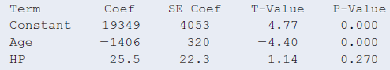
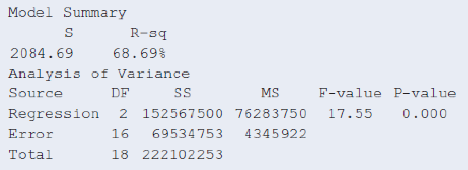
- a. Report R2 and show how it is determined by SS values in the ANOVA table.
- b. Interpret its value as a proportional reduction in prediction error.
- c. Interpret its value as the percentage of the variability in the response variable that can be explained.
Expert Solution & Answer
Want to see the full answer?
Check out a sample textbook solution
Students have asked these similar questions
Interpret the regression coefficient of X3 in relation to the Y ( X3 unit is mile)
Y = 58.286 + 13.7604 * X3
Consider the model y=-2.45x+7.18 derived from data between x=4 and x=10. What value of x represents interpolation of the data?
A regression was run to determine if there is a relationship between hours of TV watched per day (x) and
number of situps a person can do (y).
The results of the regression were:
y-ax+b
a=-0.656
b=36.681
r2-0.877969
r=-0.937
Use this to predict the number of situps a person who watches 10 hours of TV can do (to one decimal
place)
Question Help: Message instructh
Submit Question
to search
Chapter 13 Solutions
Statistics: The Art and Science of Learning From Data, Books a la Carte Edition (4th Edition)
Ch. 13.1 - Predicting weight For a study of female college...Ch. 13.1 - Prob. 2PBCh. 13.1 - Predicting college GPA For all students at Walden...Ch. 13.1 - Prob. 4PBCh. 13.1 - Does more education cause more crime? The FL Crime...Ch. 13.1 - Crime rate and income Refer to the previous...Ch. 13.1 - The economics of golf The earnings of a PGA Tour...Ch. 13.1 - Prob. 8PBCh. 13.1 - Controlling can have no effect Suppose that the...Ch. 13.1 - House selling prices Using software with the House...
Ch. 13.1 - Used cars The following data (also available from...Ch. 13.2 - Predicting sports attendance Keeneland Racetrack...Ch. 13.2 - Predicting weight Lets use multiple regression to...Ch. 13.2 - Prob. 14PBCh. 13.2 - Price of used cars For the 19 used cars listed in...Ch. 13.2 - Prob. 16PBCh. 13.2 - Softball data For the Softball data set on the...Ch. 13.2 - Slopes, correlations, and units In Example 2 on y...Ch. 13.2 - Predicting college GPA Using software with the...Ch. 13.3 - Predicting GPA For the 59 observations in the...Ch. 13.3 - Study time help GPA? Refer to the previous...Ch. 13.3 - Variability in college GPA Refer to the previous...Ch. 13.3 - Does leg press help predict body strength? Chapter...Ch. 13.3 - Prob. 24PBCh. 13.3 - Interpret strength variability Refer to the...Ch. 13.3 - Any predictive power? Refer to the previous three...Ch. 13.3 - Predicting pizza revenue Aunt Ermas Pizza...Ch. 13.3 - Prob. 28PBCh. 13.3 - Mental health again Refer to the previous...Ch. 13.3 - Prob. 30PBCh. 13.3 - House prices Use software to do further analyses...Ch. 13.4 - Body weight residuals Examples 47 used multiple...Ch. 13.4 - Strength residuals In Chapter 12, we analyzed...Ch. 13.4 - Prob. 34PBCh. 13.4 - Nonlinear effects of age Suppose you fit a...Ch. 13.4 - Prob. 36PBCh. 13.4 - Why inspect residuals? When we use multiple...Ch. 13.4 - College athletes The College Athletes data set on...Ch. 13.4 - House prices Use software with the House Selling...Ch. 13.4 - Prob. 40PBCh. 13.5 - U.S. and foreign used cars Refer to the used car...Ch. 13.5 - Prob. 42PBCh. 13.5 - Predict using house size and condition For the...Ch. 13.5 - Quality and productivity The table shows data from...Ch. 13.5 - Predicting hamburger sales A chain restaurant that...Ch. 13.5 - Prob. 46PBCh. 13.5 - House size and garage interact? Refer to the...Ch. 13.5 - Prob. 48PBCh. 13.5 - Comparing sales You own a gift shop that has a...Ch. 13.6 - Prob. 50PBCh. 13.6 - Prob. 51PBCh. 13.6 - Prob. 52PBCh. 13.6 - Prob. 53PBCh. 13.6 - Prob. 54PBCh. 13.6 - Prob. 55PBCh. 13.6 - Prob. 56PBCh. 13.6 - Prob. 57PBCh. 13.6 - Prob. 58PBCh. 13.6 - Prob. 59PBCh. 13 - House prices This chapter has considered many...Ch. 13 - Prob. 61CPCh. 13 - Prob. 62CPCh. 13 - Prob. 63CPCh. 13 - Prob. 64CPCh. 13 - Prob. 65CPCh. 13 - Prob. 66CPCh. 13 - Prob. 67CPCh. 13 - Prob. 68CPCh. 13 - Prob. 69CPCh. 13 - AIDS and AZT In a study (reported in the New York...Ch. 13 - Factors affecting first home purchase The table...Ch. 13 - Unemployment and GDP Refer to Exercise 13.67. When...Ch. 13 - Prob. 75CPCh. 13 - Prob. 76CPCh. 13 - Prob. 77CPCh. 13 - Prob. 78CPCh. 13 - Prob. 79CPCh. 13 - True or false: Slopes For data on y = college GPA,...Ch. 13 - Prob. 81CPCh. 13 - Lurking variable Give an example of three...Ch. 13 - Prob. 83CPCh. 13 - Prob. 84CPCh. 13 - Prob. 85CPCh. 13 - Logistic versus linear For binary response...Ch. 13 - Prob. 87CPCh. 13 - Prob. 88CPCh. 13 - Prob. 89CPCh. 13 - Prob. 90CPCh. 13 - Prob. 91CPCh. 13 - Prob. 92CPCh. 13 - Prob. 93CP
Knowledge Booster


Learn more about
Need a deep-dive on the concept behind this application? Look no further. Learn more about this topic, statistics and related others by exploring similar questions and additional content below.Similar questions
- For the following exercises, use Table 4 which shows the percent of unemployed persons 25 years or older who are college graduates in a particular city, by year. Based on the set of data given in Table 5, calculate the regression line using a calculator or other technology tool, and determine the correlation coefficient. Round to three decimal places of accuracyarrow_forwardFor the following exercises, consider the data in Table 5, which shows the percent of unemployed ina city of people 25 years or older who are college graduates is given below, by year. 40. Based on the set of data given in Table 6, calculate the regression line using a calculator or other technology tool, and determine the correlation coefficient to three decimal places.arrow_forwardWhat does the y -intercept on the graph of a logistic equation correspond to for a population modeled by that equation?arrow_forward
- Find the equation of the regression line for the following data set. x 1 2 3 y 0 3 4arrow_forwardTable 6 shows the population, in thousands, of harbor seals in the Wadden Sea over the years 1997 to 2012. a. Let x represent time in years starting with x=0 for the year 1997. Let y represent the number of seals in thousands. Use logistic regression to fit a model to these data. b. Use the model to predict the seal population for the year 2020. c. To the nearest whole number, what is the limiting value of this model?arrow_forwardFind Karl person's coefficient of correlation using regression coefficient byr=-0.56, bry=-0.83 Answer:arrow_forward
- The accompanying table shows results from regressions performed on data from a random sample of 21 cars. The response (y) variable is CITY (fuel consumption in mi/gal). The predictor (x) variables are WT (weight in pounds), DISP (engine displacement in liters), and HWY (highway fuel consumption in mi/gal). Which regression equation is best for predicting city fuel consumption? Why? E Click the icon to view the table of regression equations. Choose the correct answer below. O A. The equation CITY = 6.65 - 0.00161WT + 0.675HWY is best because it has a low P-value and the highest adjusted value of R2. O B. The equation CITY = 6.83 - 0.00132WT - 0.253DISP + 0.654HWY is best because it has a low P-value and the highest value of R?. OC. The equation CITY = 6.83 - 0.00132WT - 0.253DISP + 0.654HWY is best because it uses all of the available predictor variables. O D. The equation CITY = - 3.14 + 0.823HWY is best because it has a low P-value and its R2 and adjusted R? values are comparable to…arrow_forwardFor a particular red wine, the auction selling price for a 750-milliliter bottle and the age of the wine (in years) was recorded and used to regress the Auction Selling Price (the y-variable) on the Age (the x-variable). The Excel regression analysis showed that the estimated regression equation was: y with hat on top equals 9.02 plus 6.95 x Use this estimated regression equation to predict the Auction Selling Price of a 750-milliliter bottle of this red wine that is 15 years old. Give the EXACT value. The predicted Auction Selling Price of a 750-milliliter bottle of this red wine that is 15 years old is $arrow_forward
arrow_back_ios
arrow_forward_ios
Recommended textbooks for you

 Glencoe Algebra 1, Student Edition, 9780079039897...AlgebraISBN:9780079039897Author:CarterPublisher:McGraw Hill
 Functions and Change: A Modeling Approach to Coll...AlgebraISBN:9781337111348Author:Bruce Crauder, Benny Evans, Alan NoellPublisher:Cengage Learning
 Algebra & Trigonometry with Analytic GeometryAlgebraISBN:9781133382119Author:SwokowskiPublisher:Cengage
 Big Ideas Math A Bridge To Success Algebra 1: Stu...AlgebraISBN:9781680331141Author:HOUGHTON MIFFLIN HARCOURTPublisher:Houghton Mifflin Harcourt
Glencoe Algebra 1, Student Edition, 9780079039897...
Algebra
ISBN:9780079039897
Author:Carter
Publisher:McGraw Hill
Functions and Change: A Modeling Approach to Coll...
Algebra
ISBN:9781337111348
Author:Bruce Crauder, Benny Evans, Alan Noell
Publisher:Cengage Learning
Algebra & Trigonometry with Analytic Geometry
Algebra
ISBN:9781133382119
Author:Swokowski
Publisher:Cengage
Big Ideas Math A Bridge To Success Algebra 1: Stu...
Algebra
ISBN:9781680331141
Author:HOUGHTON MIFFLIN HARCOURT
Publisher:Houghton Mifflin Harcourt
Correlation Vs Regression: Difference Between them with definition & Comparison Chart; Author: Key Differences;https://www.youtube.com/watch?v=Ou2QGSJVd0U;License: Standard YouTube License, CC-BY
Correlation and Regression: Concepts with Illustrative examples; Author: LEARN & APPLY : Lean and Six Sigma;https://www.youtube.com/watch?v=xTpHD5WLuoA;License: Standard YouTube License, CC-BY