
Videos
The following data on mass rate of burning x and flame length y is representative of that which appeared in the article “Some Burning Characteristics of Filter Paper” (Combustion Science and Technology, 1971: 103–120):
| x | 1.7 | 2.2 | 2.3 | 2.6 | 2.7 | 3.0 | 3.2 |
| y | 1.3 | 1.8 | 1.6 | 2.0 | 2.1 | 2.2 | 3.0 |
| x | 3.3 | 4.1 | 4.3 | 4.6 | 5.7 | 6.1 | |
| y | 2.6 | 4.1 | 3.7 | 5.0 | 5.8 | 5.3 |
a. Estimate the parameters of a power
b. Construct diagnostic plots to check whether a power function is an appropriate model choice. c. Test H0: β = 4/3 versus Ha: β < 4/3, using a level .05 test.
d. Test the null hypothesis that states that the median flame length when burning rate is 5.0 is twice the median flame length when burning rate is 2.5 against the alternative that this is not the case.
a.
Estimate the parameters of power model.
Answer to Problem 17E
The estimate the parameters of power model are 0.626 and 1.254x.
Explanation of Solution
Given info:
The data shows the mass rate of burning x and the length of flame y.
Calculation:
The power model is given below:
Where, y is transformed into ln(y), x is transformed into ln(x).
The linear function is
The estimates of the parameters
Where,
The table below shows the calculation of estimating the parameters:
| S. No | ln(y) | ln(x) | |||
| 1 | 0.2624 | 0.5307 | 0.139256 | 0.068854 | 0.281642 |
| 2 | 0.5878 | 0.7885 | 0.46348 | 0.345509 | 0.621732 |
| 3 | 0.4701 | 0.833 | 0.391593 | 0.220994 | 0.693889 |
| 4 | 0.6932 | 0.9556 | 0.662422 | 0.480526 | 0.913171 |
| 5 | 0.742 | 0.9933 | 0.737029 | 0.550564 | 0.986645 |
| 6 | 0.7885 | 1.0987 | 0.866325 | 0.621732 | 1.207142 |
| 7 | 1.0987 | 1.1632 | 1.278008 | 1.207142 | 1.353034 |
| 8 | 0.9556 | 1.194 | 1.140986 | 0.913171 | 1.425636 |
| 9 | 1.411 | 1.411 | 1.990921 | 1.990921 | 1.990921 |
| 10 | 1.3084 | 1.4587 | 1.908563 | 1.711911 | 2.127806 |
| 11 | 1.6095 | 1.5261 | 2.456258 | 2.59049 | 2.328981 |
| 12 | 1.7579 | 1.7405 | 3.059625 | 3.090212 | 3.02934 |
| 13 | 1.6678 | 1.8083 | 3.015883 | 2.781557 | 3.269949 |
| Total | 13.3529 | 15.5016 | 18.11035 | 16.57358 | 20.22989 |
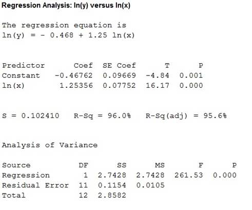
=1.253
= –0.467
Thus, the estimates of the parameters are given below:
Similarly,
b.
Construct a diagnostic plot for checking the appropriate of power model.
Answer to Problem 17E
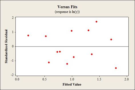
The diagnostic plot is given below:
Explanation of Solution
Calculation:
Software procedure:
Step-by-step procedure to construct a diagnostic plot is given below:
- Choose Stats>Regression> Regression.
- Select Simple and click OK
- Under Response, choose the column containing ln(y).
- Under Predictors, choose the column containing ln(x).
- Click Graphs, select residuals versus fits.
- Click OK.
Output obtained from MINITAB is given below:
The residual plot versus fitted values shows that the errors are randomly distributed with mean 0. This tells that the power model is appropriate to use for the given data.
The R-square value is 96% which tells that ln of mass rate of burning x can explain 96% of the variation in ln of flame length.
Hence, a power model is appropriate.
c.
Test the hypotheses
Answer to Problem 17E
There is sufficient evidence to conclude that
Explanation of Solution
Calculation:
That is, the slope coefficient equals to
That is, the slope coefficient is lesser than
Test statistic:
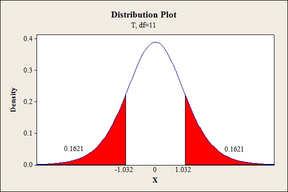
=–1.032
P-value:
Software procedure:
Step-by-step procedure to find the P-value is given below:
- Choose Graph>Probability distribution Plot>View Probability.
- Select t, enter 11 for degrees of freedom.
- Under Shaded Area tab, select X value and click on Both tails.
- Enter 1.032 for X value.
- Click OK.
Output obtained from MINITAB is given below:
Conclusion:
The P-value is 0.1621 and the level of significance is 0.05.
The P-value is greater than the level of significance is 0.05.
That is, 0.1621>0.05.
Thus, the null hypothesis is not rejected.
Thus, there is sufficient evidence to conclude that
d.
Test the hypothesis that the whether the median flame with 5.0 burning rate is twice the median flame length when the burning rate is 2.5 or not.
Answer to Problem 17E
There is no sufficient evidence to conclude the median flame with 5.0 burning rate is twice the median flame length when the burning rate is 2.5
Explanation of Solution
Calculation:
The median flame with 5.0 burning rate is twice the median flame length when the burning rate is 2.5 can be expressed as,
The hypothesis test is given below:
Test statistic:
=3.265
P-value:
Software procedure:
Step-by-step procedure to find the P-value is given below:
- Choose Graph>Probability distribution Plot>View Probability.
- Select t, enter 11 for degrees of freedom.
- Under Shaded Area tab, select X value and click on Both tails.
- Enter 3.26 for X value.
- Click OK.
Output obtained from MINITAB is given below:
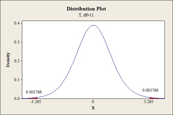
Thus, the P-value is
Conclusion:
The P-value is 0.008 and the level of significance is 0.01.
The P-value is lesser than the level of significance.
That is 0.008<0.01.
Thus, the null hypothesis is rejected.
Thus, there is no sufficient evidence to conclude the median flame with 5.0 burning rate is twice the median flame length when the burning rate is 2.5.
Want to see more full solutions like this?
Chapter 13 Solutions
Bundle: Probability And Statistics For Engineering And The Sciences, 9th + Webassign, Single-term Printed Access Card


- Given the density function f(x) = 2(1 − x), for 0 < x < 1, = 0, otherwise. Find the standard deviationarrow_forwardFind the mass of the following thin bars with the given density function. r1x2= 1 + x3, for 0 … x … 1arrow_forwardIf the measurements of the length and width of a rectangle have the joint density of f(x,y) = 1/ab for L - (a/2) < x < L + (a/2) , W - (b/2) < y < W + (b/2). and f(x,y) = 0 elsewhere, find the mean and variance of the corresponding distribution of the area of the rectangle. L for length, W for width.arrow_forward
- Let G(x,y) and H(x,y) be bivariate cdfs. Is F(x,y) = λG(x,y) + (1 −λ)H(x,y) a cdf(0 ≤λ ≤1)? Answer this question by reducing to bivariate densityarrow_forwardGiven the random variables X and Y having the following joint density: f(x, y) = 2(x + y) for 0 < y < x < 1. A) Compute the conditional pdfs: fX│Y (x) and fY│X (y). B) Are X and Y independent?arrow_forwardGiven that 0.345 of all possible observations of the variable are less than 10, determine the area under the density curve that lies to the right of 10. Given that 0.472 of all possible observation of the variable are greater than 22, determine the area under the density curve that lies to the left of 22.arrow_forward
- If the exponent of e of a bivariate normal density is −154 (x2 + 4y2 + 2xy + 2x + 8y + 4)find σ1, σ2, and ρ, given that μ1 = 0 and μ2 = −1.arrow_forwardSuppose that Y1, . . . , Yn is a random sample from a population whose density function isarrow_forwardFind the average value of the function over the given interval. f(t) = e0.03t on [0, 10]arrow_forward
- Suppose that the random variables X and Y have a joint density function given by: f(x,y)={cxy for 0≤x≤2 and 0≤y≤x, 0 otherwise c=1/2 P(X < 1), Determine whether X and Y are independentarrow_forwardThe accompanying specific gravity values for variouswood types used in construction appeared in the article“Bolted Connection Design Values Based on EuropeanYield Model” (J. of Structural Engr., 1993: 2169–2186):.31 .35 .36 .36 .37 .38 .40 .40 .40.41 .41 .42 .42 .42 .42 .42 .43 .44.45 .46 .46 .47 .48 .48 .48 .51 .54.54 .55 .58 .62 .66 .66 .67 .68 .75 Construct a stem-and-leaf display using repeatedstems, and comment on any interesting features of thedisplay.arrow_forwardFind the average value have of the function h on the given interval. h(u) = (ln(u))/u, [1, 8]arrow_forward
 MATLAB: An Introduction with ApplicationsStatisticsISBN:9781119256830Author:Amos GilatPublisher:John Wiley & Sons Inc
 Probability and Statistics for Engineering and th...StatisticsISBN:9781305251809Author:Jay L. DevorePublisher:Cengage Learning
 Statistics for The Behavioral Sciences (MindTap C...StatisticsISBN:9781305504912Author:Frederick J Gravetter, Larry B. WallnauPublisher:Cengage Learning
 Elementary Statistics: Picturing the World (7th E...StatisticsISBN:9780134683416Author:Ron Larson, Betsy FarberPublisher:PEARSON
 The Basic Practice of StatisticsStatisticsISBN:9781319042578Author:David S. Moore, William I. Notz, Michael A. FlignerPublisher:W. H. Freeman
 Introduction to the Practice of StatisticsStatisticsISBN:9781319013387Author:David S. Moore, George P. McCabe, Bruce A. CraigPublisher:W. H. Freeman