Videos
The article first introduced in Exercise 13.34 of Section 13.3 gave data on the dimensions of 27 representative food products.
- a. Use the data set given there to test the hypothesis that there is a positive linear relationship between x = minimum width and y = maximum width of an object.
- b. Calculate and interpret se.
- c. Calculate a 95% confidence interval for the mean maximum width of products with a minimum width of 6 cm.
- d. Calculate a 95% prediction interval for the maximum width of a food package with a minimum width of 6 cm.
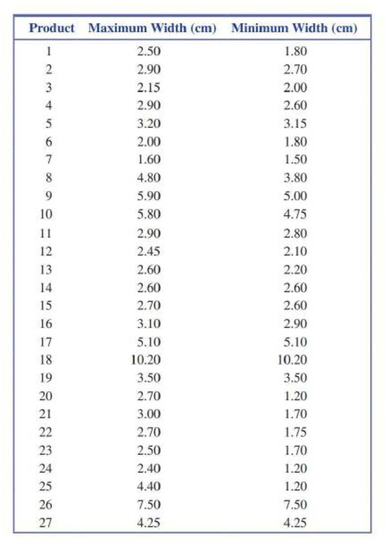
13.34 The article “Vital Dimensions in Volume Perception: Can the Eye Fool the Stomach?” (Journal of Marketing Research [1999]: 313–326) gave the accompanying data on the dimensions of 27 representative food products (Gerber baby food, Cheez Whiz, Skippy Peanut Butter, and Ahmed’s tandoori paste, to name a few).
- a. Fit the simple linear regression model that would allow prediction of the maximum width of a food container based on its minimum width.
- b. Calculate the standardized residuals (or just the residuals if a computer program that doesn’t give standardized residuals is used) and make a residual plot to determine whether there are any outliers.
- c. The data point with the largest residual is for a 1-liter Coke bottle. Delete this data point and determine the equation of the regression line. Did deletion of this point result in a large change in the equation of the estimated regression line?
- d. For the regression line of Part (c), interpret the estimated slope and, if appropriate, the intercept.
- e. For the data set with the Coke bottle deleted, are the assumptions of the simple linear regression model reasonable? Give statistical evidence.
a.
Check whether there is a positive linear relationship between minimum and maximum width of an object.
Answer to Problem 44E
There is convincing evidence that there is a positive linear relationship between minimum and maximum width of an object.
Explanation of Solution
Calculation:
The given data provide the dimensions of 27 representative food products.
1.
Here,
2.
Null hypothesis:
That is, there is no linear relationship between minimum and maximum width of an object.
3.
Alternative hypothesis:
That is, there is a positive linear relationship between minimum and maximum width of an object.
4.
Here, the significance level is
5.
Test Statistic:
The formula for test statistic is,
In the formula, b denotes the estimated slope,
6.
A standardized residual plot is shown below.
Standardized residual values and standardized residual plot:
Software procedure:
Step-by-step procedure to compute standardized residuals and its plot using MINITAB software:
- Select Stat > Regression > Regression > Fit Regression Model
- In Response, enter the column of Maximum width.
- In Continuous Predictors, enter the columns of Minimum width.
- In Graphs, select Standardized under Residuals for Plots.
- In Results, select for all observations under Fits and diagnostics.
- In Residuals versus the variables, select Minimum width.
- Click OK.
Output obtained the MINTAB software is given below:
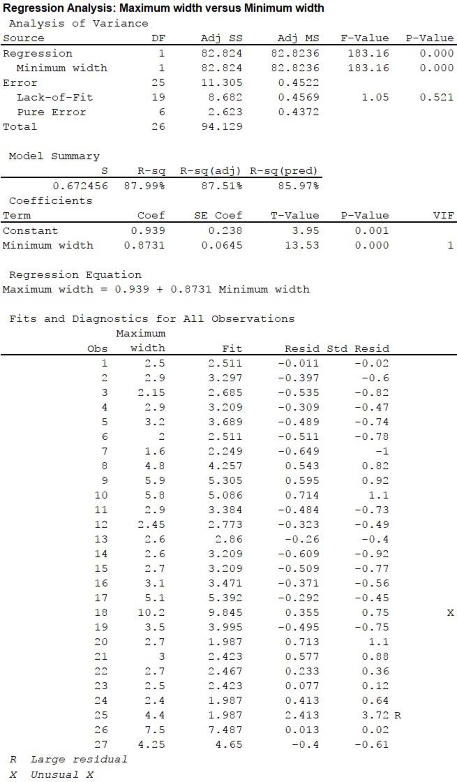
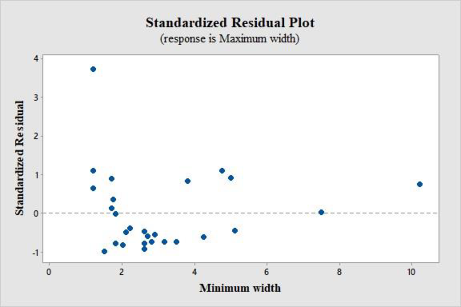
From the standardized residual plot, it is observed that one point lies outside the horizontal band of 3 units from the central line of 0. The standardized residual for this outlier is 3.72, which is for the product 25.
Assumption:
Here, the assumption made is that, the simple linear regression model is appropriate for the data, even though there is one extreme standardized residual.
7.
Calculation:
Test Statistic:
In the MINITAB output, the test statistic value is displayed in the column “T-value” corresponding to “Minimum width”, in the section “Coefficients”. The value is 13.53.
8.
P-value:
From the above output, the correponding P-value is 0.
9.
Rejection rule:
If
Conclusion:
The P-value is 0.
The level of significance is 0.05.
The P-value is less than the level of significance.
That is,
Based on the rejection rule, reject the null hypothesis.
Thus, there is convincing evidence that there is a positive linear relationship between minimum and maximum width of an object.
b.
Compute and interpret
Answer to Problem 44E
Explanation of Solution
Calculation:
From the MINITAB output in Part (a), it is clear that
On an average, there is a 67.246% deviation of the maximum width in the sample from the value predicted by least-squares regression.
c.
Find the 95% confidence interval for the mean maximum width of products, for a minimum width of 6 cm.
Answer to Problem 44E
The 95% interval for the mean maximum width of products, for a minimum width of 6 cm is (5.708, 6.647).
Explanation of Solution
Calculation:
The confidence interval for
From the MINITAB output in Part (a), the estimated linear regression line is
Point estimate:
The point estimate is calculated as follows.
Estimated standard deviation:
For the given x values, the summation values are given in the following table.
| Minimum width (X) | |
| 1.8 | 3.24 |
| 2.7 | 7.29 |
| 2 | 4 |
| 2.6 | 6.76 |
| 3.15 | 9.9225 |
| 1.8 | 3.24 |
| 1.5 | 2.25 |
| 3.8 | 14.44 |
| 5 | 25 |
| 4.75 | 22.5625 |
| 2.8 | 7.84 |
| 2.1 | 4.41 |
| 2.2 | 4.84 |
| 2.6 | 6.76 |
| 2.6 | 6.76 |
| 2.9 | 8.41 |
| 5.1 | 26.01 |
| 10.2 | 104.04 |
| 3.5 | 12.25 |
| 1.2 | 1.44 |
| 1.7 | 2.89 |
| 1.75 | 3.0625 |
| 1.7 | 2.89 |
| 1.2 | 1.44 |
| 1.2 | 1.44 |
| 7.5 | 56.25 |
| 4.25 | 18.0625 |
The value of
Substitute,
Formula for Degrees of freedom:
The formula for degrees of freedom is,
The number of data values given is 27, that is
Critical value:
From the Appendix: Table of t Critical Values:
- Locate the value 25 in the degrees of freedom (df) column.
- Locate the 0.95 in the row of central area captured.
- The intersecting value that corresponds to the df 25 with confidence level 0.95 is 2.060.
Thus, the critical value for
Substitute,
Therefore, one can be 95% confident that the mean maximum width of products with a minimum width of 6 cm will be between 5.708 cm and 6.647 cm.
d.
Find a 95% prediction interval for the mean maximum width of products with a minimum width of 6 cm.
Answer to Problem 44E
The 95% prediction interval for the mean maximum width of products with a minimum width of 6 cm is (4.716, 7.640).
Explanation of Solution
Calculation:
The confidence interval for
The estimated standard deviation of the amount by which a single y observation deviates from the value predicted by an estimated regression line is,
Substitute
From Part (c), the critical value for
Substitute,
Therefore, the 95% prediction interval for the mean maximum width of products with a minimum width of 6 cm is (4.716, 7.640).
Want to see more full solutions like this?
Chapter 13 Solutions
Introduction To Statistics And Data Analysis


- 1. The following table illustrates the BMI for a number of patients recently enrolled in a study investigating the relationship between BMI and type 2 diabetes. Participant BMI (kg/m2) A 26.5 B 19.2 C 29.7 D 27.4 E 30.2 F 28.9 A) Assuming the participants can be considered to be normally distributed, and that they comefrom a population with a σ=2.4 kg/m2, calculate a 95% confidence interval for the mean BMI ofthe population for which they represent.B) Correctly interpret the confidence interval you found above.arrow_forwardA U.S. Food Survey showed that Americans routinely eat beef in their diet. Suppose that in a study of 49 consumers in Illinois and 64 consumers in Texas the following results were obtained from two samples regarding average yearly beef consumption: Illinois Texas = 49 = 64 = 54.1lb = 60.4lb S1 = 7.0 S2 = 8.0 Develop a 95% confidence Interval Estimate for the difference between the two population means.arrow_forwardIn Exercises, presume that the assumptions for regression inferences are met.Crown-Rump Length. Following are the data on age of fetuses and length of crown-rump from Exercise. x 10 10 13 13 18 19 19 23 25 28 y 66 66 108 106 161 166 177 228 235 280 a. Determine a point estimate for the mean crown-rump length of all 19-week-old fetuses.b. Find a 90% confidence interval for the mean crown-rump length of all 19-week-old fetuses.c. Find the predicted crown-rump length of a 19-week-old fetus.d. Determine a 90% prediction interval for the crown-rump length of a 19-week-old fetus.ExerciseApplying the Concepts and SkillsIn Exercises, we repeat the information from Exercises. For each exercise here, discuss what satisfying Assumptions 1–3 for regression inferences by the variables under consideration would mean.arrow_forward
- In exercise 7, the data on y = annual sales ($1000s) for new customer accounts andx = number of years of experience for a sample of 10 salespersons provided the estimatedregression equation yˆ = 80 + 4x. For these data x = 7, o(xi − x)2 = 142, and s = 4.6098.a. Develop a 95% confidence interval for the mean annual sales for all salespersons withnine years of experience.b. The company is considering hiring Tom Smart, a salesperson with nine years of experience.Develop a 95% prediction interval of annual sales for Tom Smart.c. Discuss the differences in your answers to parts (a) and (b).arrow_forwardFind the critical value z a/2 that corresponds to the given confidence level 96arrow_forward11.36 Use the data from Exercise 11.22.a. Estimate the mean time to run 10 km for athletes having a treadmill time of11 minutes.b. Place a 95% confidence interval on the mean time to run 10 km for athleteshaving a treadmill time of 11 minutes.arrow_forward
- Find the critical z⋆z⋆ for a level 96.38 % confidence interval.arrow_forwardExercise #1 Open the Excel worksheet MPGDATA.XLS from Blackboard>Excel #5 Files. The data in column A of this worksheet represent the miles per gallon gasoline consumption for a random sample of 55 makes and models of passenger cars (source: Environmental Protection Agency) Use the Excel Confidence Interval Template to: Construct a 95% confidence interval for the population mean miles per gallon consumption for passenger cars. Use the Excel Hypothesis Testing Template to: Test the hypothesis that the population mean of miles per gallon gasoline consumption for passenger cars is different from 25 mpg. Use a significance level of 5%. Do we know ? for the mpg consumption? Can we use the normal distribution for the hypothesis test? State the null and alternative hypotheses. Perform the appropriate test and print the output. Look at the p-value in the output. Compare it to ?. Do we reject the null hypothesis or not? Generate the descriptive statistics (mean, standard…arrow_forwardThe cost of making a batch of a certain product depends on the size of the batch, as shown by the following sample data: Cost $ 30 70 140 270 530 1010 2000 5100 size of the batch 1 5 10 25 50 100 250 500 a) Fit a straight line to said data, with the least squares method, use the lot size as the independent variable. b) Find a 95% confidence interval for alfa that can be interpreted as the fixed overhead cost of manufacture.arrow_forward
- In simple linear regression, at what value of the independent variable, X, will the 95% confidence interval for the average value of Y be narrowest? At what value will the 95% prediction interval for the value of Y for a single n ew observation be narrowest?arrow_forwardThe table below contains summary statistics about the trading density (sales per square metre, R/m2) for two random and independent samples of 18 housing developments in the Western Cape, and 13 housing developments in the Free State. Assume that the trading densities of the Western Cape and the Free State housing developments are normally distributed. Housing cost Western cape Free state Sample mean (R) 2500.2 2100.7 Sample standard deviation (R) 820.3 694.6 a. Estimate a 95% confidence interval for the standard deviation of the cost of housing developments in the Free State. b. Are the variances of the trading densities of housing developments in the Western Cape and the Free State are the same? Test at the 10% level. (Note: In answering this question, make sure you state the following: null and alternative hypotheses, test statistic and critical value. Write your final answers to 3 decimal places).c. Estimate a 90% confidence interval for the difference between the mean…arrow_forwardfor a sample size of 12 and a 90% confidence interval, the t statistic used to estimate U would be.arrow_forward
 MATLAB: An Introduction with ApplicationsStatisticsISBN:9781119256830Author:Amos GilatPublisher:John Wiley & Sons Inc
 Probability and Statistics for Engineering and th...StatisticsISBN:9781305251809Author:Jay L. DevorePublisher:Cengage Learning
 Statistics for The Behavioral Sciences (MindTap C...StatisticsISBN:9781305504912Author:Frederick J Gravetter, Larry B. WallnauPublisher:Cengage Learning
 Elementary Statistics: Picturing the World (7th E...StatisticsISBN:9780134683416Author:Ron Larson, Betsy FarberPublisher:PEARSON
 The Basic Practice of StatisticsStatisticsISBN:9781319042578Author:David S. Moore, William I. Notz, Michael A. FlignerPublisher:W. H. Freeman
 Introduction to the Practice of StatisticsStatisticsISBN:9781319013387Author:David S. Moore, George P. McCabe, Bruce A. CraigPublisher:W. H. Freeman