
Concept explainers
a.
Find the regression equation.
a.
Answer to Problem 25CE
The regression equation is
Explanation of Solution
Calculation:
Multiple linear regression model:
A multiple linear regression model is given as
Here, a is the intercept term of the regression model, that is, the value of predicted value of y when X’s are 0 and
In the given part the predicted dependent variable y is the monthly salary and the length of service
Step by step procedure to obtain the regression equation using MINITAB software:
- Choose Stat > Regression > Regression > Fit Regression Model.
- Under Responses, enter the column of Salary.
- Under Continuous predictors, enter the columns of Service, Age, Gender and Job.
- Click OK.
Output using MINITAB software is given below:
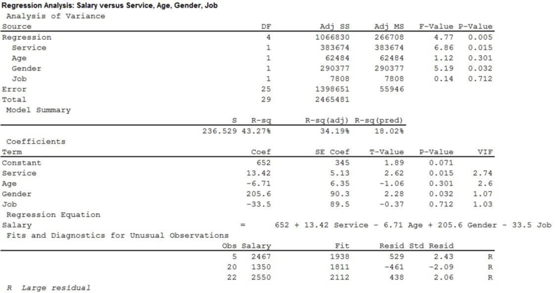
Thus, the regression equation is
b.
Find the value of
Also explain about the
b.
Answer to Problem 25CE
The value of
Explanation of Solution
According to output in Part (a), the value of
Hence, it can be said that only 43.27% variability in the monthly salary is explained by the length of service, age, gender and the job designation of the employees, using the regression equation.
c.
Perform a global test to find whether any of the independent variables are different from 0.
c.
Answer to Problem 25CE
There is enough evidence that any of the independent variables are different from 0 at 0.05 significance level.
Explanation of Solution
Calculation:
Consider that y is dependent variable and
State the hypotheses:
Null hypothesis:
That is, the model is not significant.
Alternative hypothesis:
That is, the model is significant.
In case of global test the F test statistic is defined as,
According to the output from Part (a) the value of F statistic is 4.77 with numerator degrees of freedom 4 and denominator degrees of freedom 25.
Consider that, the level of significance is
Decision rule:
- If
- Otherwise failed to reject the null hypothesis.
Conclusion:
Here, p-value corresponding to the global test is 0.
Hence,
That is, the p-value is less than the level of significance.
Therefore, reject the null hypothesis.
Hence, it can be concluded that any of the independent variables are different from 0 at 0.05 significance level.
d.
Perform an individual test to determine whether any of the independent variables can be dropped.
d.
Answer to Problem 25CE
There is no significant relationship between the dependent variable “Salary” and the independent variables “Age” and “Job”, thus it is better to omit these two variables.
Explanation of Solution
Calculation:
For independent variable
Consider that
State the hypotheses:
Null hypothesis:
That is, there is no significant relationship between y and
Alternative hypothesis:
That is, there is significant relationship between y and
In case of individual regression coefficient test the t test statistic is defined as,
According to the output in Part (a) the t statistic value corresponding to
Conclusion:
Here, p-value corresponding to the “Service”
Hence,
That is, the p-value is less than the level of significance.
Therefore, reject the null hypothesis.
Hence, it can be concluded that there is significant relationship between y and
For independent variable
Consider that
State the hypotheses:
Null hypothesis:
That is, there is no significant relationship between y and
Alternative hypothesis:
That is, there is significant relationship between y and
According to the output in Part (a) the value of t test statistic corresponding to
Conclusion:
Here, p-value corresponding to the “Age”
Hence,
That is, the p-value is greater than the level of significance.
Therefore, fail to reject the null hypothesis.
Hence, it can be concluded that there is no significant relationship between y and
For independent variable
Consider that
State the hypotheses:
Null hypothesis:
That is, there is no significant relationship between y and
Alternative hypothesis:
That is, there is significant relationship between y and
According to the output in Part (d) the value of t test statistic corresponding to
Conclusion:
Here, p-value corresponding to the “Gender”
Hence,
That is, the p-value is less than the level of significance.
Therefore, reject the null hypothesis.
Hence, it can be concluded that there is significant relationship between y and
For independent variable
Consider that
State the hypotheses:
Null hypothesis:
That is, there is no significant relationship between y and
Alternative hypothesis:
That is, there is significant relationship between y and
According to the output in Part (a) the value of t test statistic corresponding to
Conclusion:
Here, p-value corresponding to the “Job”
Hence,
That is, the p-value is greater than the level of significance.
Therefore, fail to reject the null hypothesis.
Hence, it can be concluded that there is no significant relationship between y and
As there is no significant relationship between the dependent variable “Salary” and the independent variables “Age” and “Job”, thus it is better to omit these two variables and perform the regression analysis only with the independent variables “Service” and “Gender”.
e.
Find the regression equation using the significant independent variables.
Find the amount of money does a man earn per month than a woman.
Explain whether there is any difference
e.
Answer to Problem 25CE
The regression equation is
Explanation of Solution
Calculation:
Dummy variable:
A dichotomous variable is defined as a dummy variable, where one outcome is defined as 1 another as 0.
In the Part the predicted dependent variable y is the monthly salary and the length of service
The independent random variable
Hence,
Step by step procedure to obtain the regression equation using MINITAB software:
- Choose Stat > Regression > Regression > Fit Regression Model.
- Under Responses, enter the column of Salary.
- Under Continuous predictors, enter the columns of Service, and Gender.
- Click OK.
Output using MINITAB software is given below:
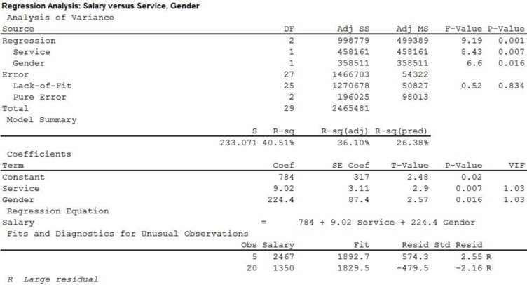
Thus, the regression equation is
Here, the coefficient of
As there is no significant relationship between the monthly salary and the designation of the employees, hence whether the employee has a management or engineering position does not make any difference.
Want to see more full solutions like this?
Chapter 14 Solutions
STATISTICAL TECHNIQUES FOR BUSINESS AND


 Mathematics For Machine TechnologyAdvanced MathISBN:9781337798310Author:Peterson, John.Publisher:Cengage Learning,
 Holt Mcdougal Larson Pre-algebra: Student Edition...AlgebraISBN:9780547587776Author:HOLT MCDOUGALPublisher:HOLT MCDOUGAL