Concept explainers
Videos
The following is the ANOVA summary table for a multiple regression model with two independent variables:
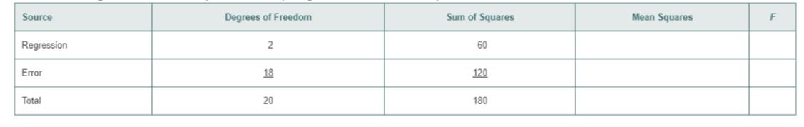
a determine whether there is a significant relationship between
b. compute the coefficients of partial determination,
Want to see the full answer?
Check out a sample textbook solution
Chapter 14 Solutions
BASIC BUSINESS STATISTICS-STUD.SOLN.MAN


- Olympic Pole Vault The graph in Figure 7 indicates that in recent years the winning Olympic men’s pole vault height has fallen below the value predicted by the regression line in Example 2. This might have occurred because when the pole vault was a new event there was much room for improvement in vaulters’ performances, whereas now even the best training can produce only incremental advances. Let’s see whether concentrating on more recent results gives a better predictor of future records. (a) Use the data in Table 2 (page 176) to complete the table of winning pole vault heights shown in the margin. (Note that we are using x=0 to correspond to the year 1972, where this restricted data set begins.) (b) Find the regression line for the data in part ‚(a). (c) Plot the data and the regression line on the same axes. Does the regression line seem to provide a good model for the data? (d) What does the regression line predict as the winning pole vault height for the 2012 Olympics? Compare this predicted value to the actual 2012 winning height of 5.97 m, as described on page 177. Has this new regression line provided a better prediction than the line in Example 2?arrow_forwardFor the following exercises, use Table 4 which shows the percent of unemployed persons 25 years or older who are college graduates in a particular city, by year. Based on the set of data given in Table 5, calculate the regression line using a calculator or other technology tool, and determine the correlation coefficient. Round to three decimal places of accuracyarrow_forwardFor the following exercises, consider the data in Table 5, which shows the percent of unemployed in a city ofpeople25 years or older who are college graduates is given below, by year. 41. Based on the set of data given in Table 7, calculatethe regression line using a calculator or othertechnology tool, and determine the correlationcoefficient to three decimal places.arrow_forward
- For the following exercises, consider the data in Table 5, which shows the percent of unemployed ina city of people 25 years or older who are college graduates is given below, by year. 40. Based on the set of data given in Table 6, calculate the regression line using a calculator or other technology tool, and determine the correlation coefficient to three decimal places.arrow_forwardXYZ Corporation Stock Prices The following table shows the average stock price, in dollars, of XYZ Corporation in the given month. Month Stock price January 2011 43.71 February 2011 44.22 March 2011 44.44 April 2011 45.17 May 2011 45.97 a. Find the equation of the regression line. Round the regression coefficients to three decimal places. b. Plot the data points and the regression line. c. Explain in practical terms the meaning of the slope of the regression line. d. Based on the trend of the regression line, what do you predict the stock price to be in January 2012? January 2013?arrow_forwardLife Expectancy The following table shows the average life expectancy, in years, of a child born in the given year42 Life expectancy 2005 77.6 2007 78.1 2009 78.5 2011 78.7 2013 78.8 a. Find the equation of the regression line, and explain the meaning of its slope. b. Plot the data points and the regression line. c. Explain in practical terms the meaning of the slope of the regression line. d. Based on the trend of the regression line, what do you predict as the life expectancy of a child born in 2019? e. Based on the trend of the regression line, what do you predict as the life expectancy of a child born in 1580?2300arrow_forward
- Given below are results from the regression analysis where the dependent variable is the number of weeks a worker is unemployed due to a layoff (Unemploy) and the independent variables are the age of the worker (Age), the number of years of education received (Edu), the number of years at the previous job (Job Yr), a dummy variable for marital status (Married: 1=married, 0=otherwise), a dummy variable for head of household (Head: 1=yes, 0=no) and a dummy variable for management position (Manager: 1=yes, 0=no). We shall call this Model 1. The coefficient of partial determination (R2Yj.(All variables except j)) of each of the six predictors are, respectively, 0.2807, 0.0386, 0.0317, 0.0141, 0.0958, and 0.1201. Model 2 is the regression analysis where the dependent variable is Unemploy and the independent variables are Age and Manager. The results of the regression analysis are given. Refer to model 1. Which of the following is the correct null hypothesis to test…arrow_forwardThe accompanying data represent the weights of various domestic cars and their gas mileages in the city. The linear correlation coefficient between the weight of a car and its miles per gallon in the city is r= - 0.984. The least-squares regression line treating weight as the explanatory variable and miles per gallon as the response variable is y = - 0.0066x + 43.3954. Complete parts (a) and (b) below. Click the icon to view the data table. (a) What proportion of the variability in miles per gallon is explained by the relation between weight of the car and miles per gallon? Data Table The proportion of the variability in miles per gallon explained by the relation between weight of the car and miles per gallon is %. (Round to one decimal place as needed.) (b) Interpret the coefficient of determination. Full data set % of the variance in is by the linear model. Miles per Miles per Weight (pounds), x Weight (pounds), x Car Car (Round to one decimal place as needed.) Gallon, y Gallon, y…arrow_forwardThe accompanying data represent the weights of various domestic cars and their gas mileages in the city. The linear correlation coefficient between the weight of a car and its miles per gallon in the city is r= - 0.972. The least-squares regression line treating weight as the explanatory variable and miles per gallon as the response variable is y= - 0.0070x + 44.4405. Complete parts (a) and (b) below. Click the icon to view the data table. ..... (a) What proportion of the variability in miles per gallon is explained by the relation between weight of the car and miles per gallon? The proportion of the variability in miles per gallon explained by the relation between weight of the car and miles per gallon is %. (Round to one decimal place as needed.) (b) Interpret the coefficient of determination. % of the variance in is by the linear model. Data Table (Round to one decimal p Full data set gas mileage Miles per Weight (pounds), x Weight (pounds), x Miles per Gallon, y Car Car Gallon, y…arrow_forward
- b. What does the scatter diagram developed in part (a) indicate about the relationship between the two variables? The scatter diagram indicates a positive ✔✔✔ linear relationship between the hotel room rate and the amount spent on entertainment. c. Develop the least squares estimated regression equation. Entertainment = 18.2594 X + 1.0272 Room Rate (to 4 decimals) d. Provide an interpretation for the slope of the estimated regression equation (to 3 decimals). The slope of the estimated regression line is approximately 1.027 So, for every dollar increase ♥ e. The average room rate in Chicago is $128, considerably higher than the U.S. average. Predict the entertainment expense per day for Chicago (to whole number). $ 150 in the hotel room rate the amount spent on entertainment increases by $1.027arrow_forwardAs a marketing manager for TriFood, you want to determine whether store Sales (# sold in one month) of TriPower bars are related to price (in cents) of TriPower bars and in-store promotional expenditures (in dollars) for TriPower bars. You conduct a multiple regression analysis with store Sales (Y) as the response variable, and Price (X1) and Promotion (X2) as explanatory variables. Use the pictured Excel regression output below to answer the questions. a) Interpret the value for R square. Interpret the estimated coefficient for price. b) State the hypotheses for assessing the statistical significance of the overall regression equation. Does the model overall fit the data (yes or no?) f) An external consultant to TriFoods believes that for every $1 increase in promotional expenditures, sales will increase by 4.7 units. Test the consultant's hypothesis at a 5% significance level using both approaches (tcalc vs tcrit and p-value vs a).arrow_forwardAs a marketing manager for TriFood, you want to determine whether store Sales (# sold in one month) of TriPower bars are related to price (in cents) of TriPower bars and in-store promotional expenditures (in dollars) for TriPower bars. You conduct a multiple regression analysis with store Sales (Y) as the response variable, and Price (X1) and Promotion (X2) as explanatory variables. Use the pictured Excel regression output below to answer the questions. a) Write the estimated multiple regression equation. b) Should one interpret the estimated value for the intercept (yes or no)? c) Interpret the value for Standard Error under Regression Statistics. d) Interpret the value for R square. e) State the hypotheses for assessing the statistical significance of the overall regression equation. f) Interpret the estimated coefficient for price. g) An external consultant to TriFoods believes that for every $1 increase in promotional expenditures, sales will increase by 4.7 units. Test the…arrow_forward
 Glencoe Algebra 1, Student Edition, 9780079039897...AlgebraISBN:9780079039897Author:CarterPublisher:McGraw Hill
 Functions and Change: A Modeling Approach to Coll...AlgebraISBN:9781337111348Author:Bruce Crauder, Benny Evans, Alan NoellPublisher:Cengage Learning
 Algebra & Trigonometry with Analytic GeometryAlgebraISBN:9781133382119Author:SwokowskiPublisher:Cengage
 Linear Algebra: A Modern IntroductionAlgebraISBN:9781285463247Author:David PoolePublisher:Cengage Learning