
Videos
a.
Test for main effects and interactions at
a.
Answer to Problem 75SE
Main effect of factor A is significant.
Main effect of factor B is not significant.
The interaction is significant.
Explanation of Solution
Calculation:
The data represents the two factorial experiments to investigate the effect of pH and catalyst concentration on product viscosity.
Factor A is pH and Factor B is Catalyst Concentration.
State the hypotheses:
Main effect of factor A:
Null hypothesis:
Alternative hypothesis:
Main effect of factor B:
Null hypothesis:
Alternative hypothesis:
Interaction effect of Factor A and B:
Null hypothesis:
Alternative hypothesis:
Step-by-step procedure to find the factorial design table is as follows:
Software procedure:
- Choose Stat > DOE > Factorial > Create Factorial Design.
- Under Type of Design, choose General full factorial design.
- From Number of factors, choose 2.
- Click Designs.
- In Factor A, type A under Name and type 2 Under Number of Levels.
- In Factor B, type B under Name and type 2 Under Number of Levels.
- From Number of replicates, choose 4.
- Click OK.
- Select Summary table under Results.
- Click OK.
- Enter the corresponding response in the newly created factorial design worksheet.
Step-by-step procedure for finding the ANOVA table is as follows:
- Choose Stat > DOE > Factorial > Analyze Factorial Design.
- In Response, enter Responses.
- In Terms, select all the terms.
- In Results, choose “Model summary and ANOVA table”.
- Click OK in all the dialog boxes.
Output obtained by MINITAB procedure is as follows:
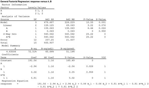
For Factor A, the F-test statistic is 6.44 and the p-value is 0.026.
For Factor B, the F-test statistic is 0.00 and the p-value is 0.958.
For interaction, the F-test statistic is 25.22 and the p-value is 0.00.
Decision:
If
If
Conclusion:
Factor A:
Here, the P-value is less than the level of significance.
That is,
Therefore, the null hypothesis is rejected.
Thus, Main effect of factor A is significant at
Factor B:
Here, the P-value is greater than the level of significance.
That is,
Therefore, the null hypothesis is not rejected.
Thus, Main effect of factor B is not significant at
Interaction:
Here, the P-value is less than the level of significance.
That is,
Therefore, the null hypothesis is rejected.
Thus, the interaction is significant at
Thus, it can be concluded that:
Main effect of factor A is significant.
Main effect of factor B is not significant.
The interaction is significant.
b.
Graphically analyze the interaction.
b.
Answer to Problem 75SE
The interaction plot indicates that there is a strong interaction.
Explanation of Solution
Calculation:
Software procedure:
Step by step procedure to obtain normal plot and residual plot using Minitab software is given as,
- Choose Stat > DOE > Factorial > Factorial plot.
- In Interaction select setup.
- In Response, enter Responses.
- In Factor included plots, select AA,BB.
- In Types of means to use in plot, choose Data means..
- Click OK.
Output using the MINITAB software is given below:
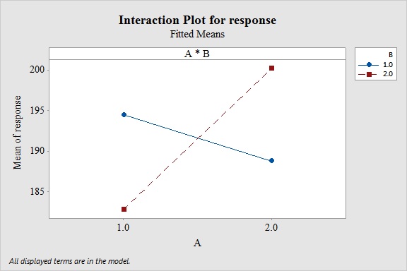
Interpretation:
From the interaction plot it is clear that when Factor A is at low level, the response is large for the lower values of B and is small at the high level of B. Similarly, if Factor A is at high level, the response is small for the higher values of B and is higher at the smallest level of B.
Thus, the interaction plot indicates that there is a strong interaction.
c.
Analyze the residuals from the experiment.
c.
Answer to Problem 75SE
The residuals are acceptable and normality assumption is not reasonable.
Explanation of Solution
Justification:
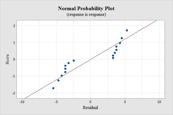
The conditions for a residual plot and normal plot that is well fitted for the data are,
- There should not any bend, which would violate the straight enough condition.
- There must not any outlier, which, were not clear before.
- There should not any change in the spread of the residuals from one part to another part of the plot.
Software procedure:
Step by step procedure to obtain normal plot and residual plot using Minitab software is given as,
- Choose Stat > DOE > Factorial > Analyze Factorial Design.
- In Response, enter Responses.
- In Terms, select all the terms.
- In Results, choose “Model summary and ANOVA table”.
- In Confidence level, enter 0.95.
- In residual plots select Normal plot of residuals, Residual versus fits.
- In residual versus the variables enter the column of Factor A and Factor B.
- Click OK.
Output using the MINITAB software is given below:
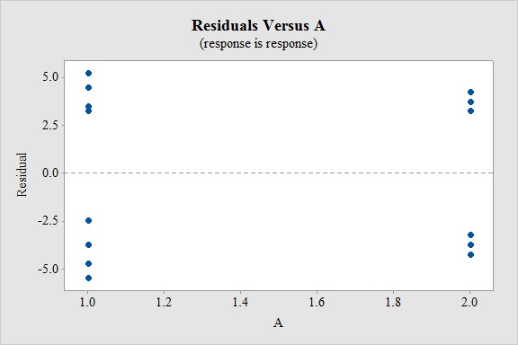
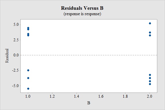
Interpretation:
In normal probability plot, the points do not lie along the straight line and there is a gap in the middle of the normal probability plot. Thus, normality assumption is not satisfied. There is no much variability for the variables.
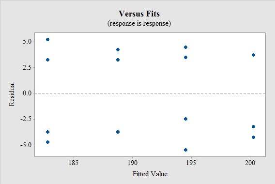
Also, there is no change in the spread of the residuals from one part to another part of the residual plot.
Thus, the residuals are acceptable and normality assumption is not reasonable.
Want to see more full solutions like this?
Chapter 14 Solutions
Applied Statistics and Probability for Engineers


 MATLAB: An Introduction with ApplicationsStatisticsISBN:9781119256830Author:Amos GilatPublisher:John Wiley & Sons Inc
 Probability and Statistics for Engineering and th...StatisticsISBN:9781305251809Author:Jay L. DevorePublisher:Cengage Learning
 Statistics for The Behavioral Sciences (MindTap C...StatisticsISBN:9781305504912Author:Frederick J Gravetter, Larry B. WallnauPublisher:Cengage Learning
 Elementary Statistics: Picturing the World (7th E...StatisticsISBN:9780134683416Author:Ron Larson, Betsy FarberPublisher:PEARSON
 The Basic Practice of StatisticsStatisticsISBN:9781319042578Author:David S. Moore, William I. Notz, Michael A. FlignerPublisher:W. H. Freeman
 Introduction to the Practice of StatisticsStatisticsISBN:9781319013387Author:David S. Moore, George P. McCabe, Bruce A. CraigPublisher:W. H. Freeman