
Concept explainers
Videos
Find the values of k, which correspond to the useful model at the 0.05 level of significance.
Explain the large value of
Answer to Problem 32E
The values of k less than 9 corresponds to the useful model at the 0.05 level of significance.
Explanation of Solution
Calculation:
It is given that the sample size (n) is 15 and the value of
Test statistic:
Where, n is the sample size and k is the number of variables in the model.
The value of F test statistic is calculated as follows:
For
The value of F test statistic is calculated as follows:
P-value:
Software procedure:
Step-by-step procedure to find the P-value using the MINITAB software:
- Choose Graph > Probability Distribution Plot choose View Probability > OK.
- From Distribution, choose ‘F’ distribution.
- Enter the Numerator df as 1 and Denominator df as 13.
- Click the Shaded Area tab.
- Choose Probability Value and Right Tail for the region of the curve to shade.
- Enter the Probability value as 0.05.
- Click OK.
Output obtained using the MINITAB software is represented as follows:
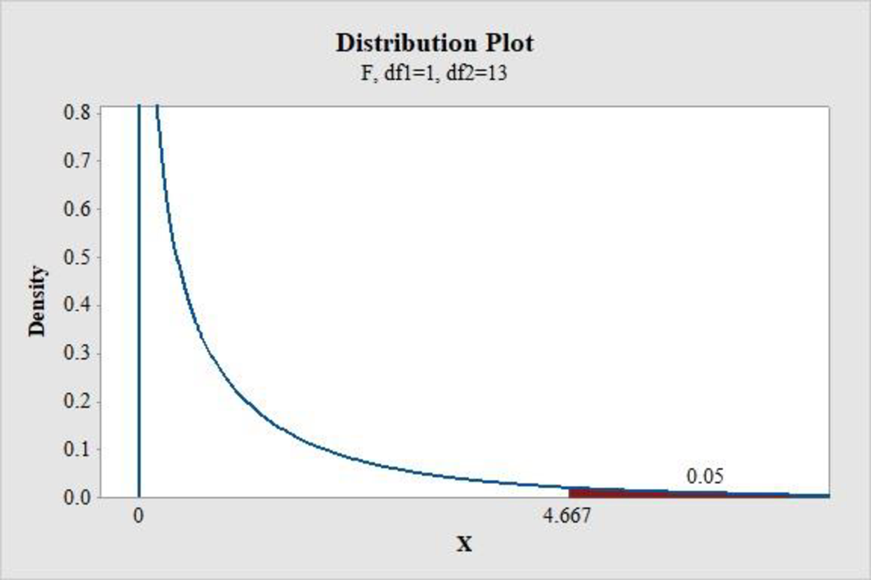
From the MINITAB output, the critical value is 4.667.
Conclusion:
If the F test statistic value is greater than the critical value, then reject the null hypothesis.
Therefore, the F test statistic of 117 is greater than the critical value of 4.667.
Hence, reject the null hypothesis.
Thus, there is convincing evidence that the model is useful.
For
The value of F test statistic is calculated as follows:
P-value:
Software procedure:
Step-by-step procedure to find the P-value using the MINITAB software:
- Choose Graph > Probability Distribution Plot choose View Probability > OK.
- From Distribution, choose ‘F’ distribution.
- Enter the Numerator df as 2 and Denominator df as 12.
- Click the Shaded Area tab.
- Choose Probability Value and Right Tail for the region of the curve to shade.
- Enter the Probability value as 0.05.
- Click OK.
Output obtained using the MINITAB software is represented as follows:
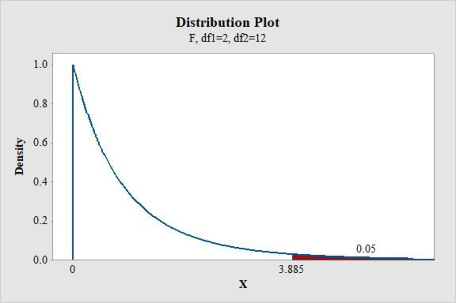
From the MINITAB output, the critical value is 3.885.
Conclusion:
If the F test statistic value is greater than the critical value, then reject the null hypothesis.
Therefore, the F test statistic of 54 is greater than the critical value of 3.885.
Hence, reject the null hypothesis.
Thus, there is convincing evidence that the model is useful.
For
The value of F test statistic is calculated as follows:
P-value:
Software procedure:
Step-by-step procedure to find the P-value using the MINITAB software:
- Choose Graph > Probability Distribution Plot choose View Probability > OK.
- From Distribution, choose ‘F’ distribution.
- Enter the Numerator df as 3 and Denominator df as 11.
- Click the Shaded Area tab.
- Choose Probability Value and Right Tail for the region of the curve to shade.
- Enter the Probability value as 0.05.
- Click OK.
Output obtained using the MINITAB software is represented as follows:
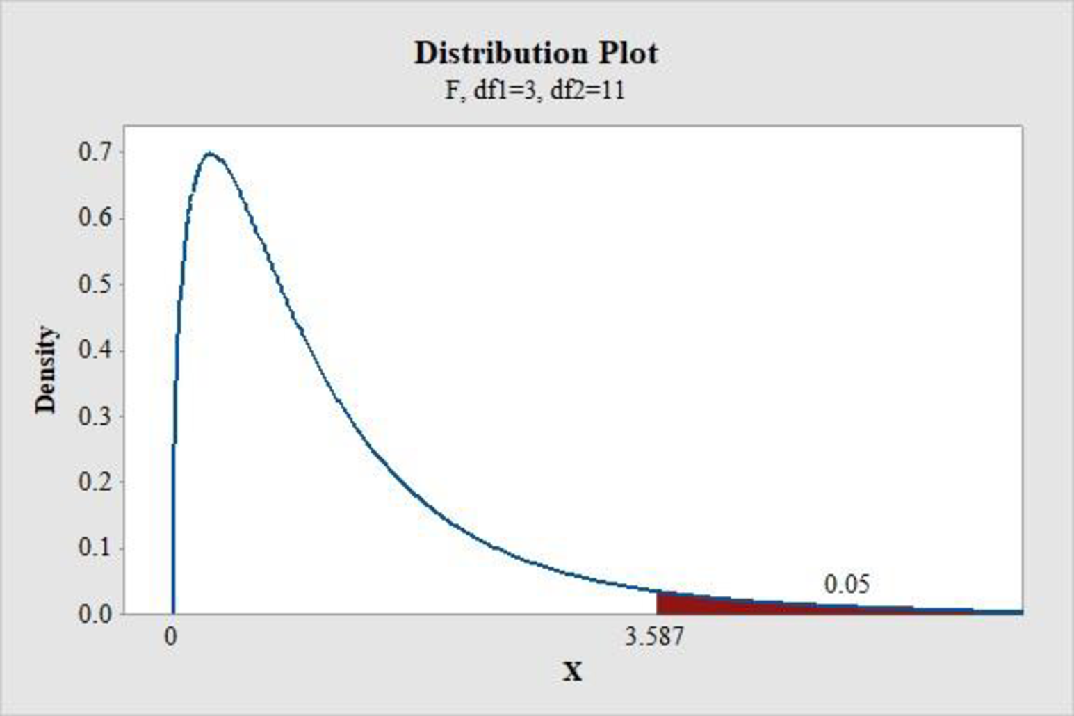
From the MINITAB output, the critical value is 3.587.
Conclusion:
If the F test statistic value is greater than the critical value, then reject the null hypothesis.
Therefore, the F test statistic of 33 is greater than the critical value of 3.587.
Hence, reject the null hypothesis.
Thus, there is convincing evidence that the model is useful.
For
The value of F test statistic is calculated as follows:
P-value:
Software procedure:
Step-by-step procedure to find the P-value using the MINITAB software:
- Choose Graph > Probability Distribution Plot choose View Probability > OK.
- From Distribution, choose ‘F’ distribution.
- Enter the Numerator df as 5 and Denominator df as 9.
- Click the Shaded Area tab.
- Choose Probability Value and Right Tail for the region of the curve to shade.
- Enter the Probability value as 0.05.
- Click OK.
Output obtained using the MINITAB software is represented as follows:
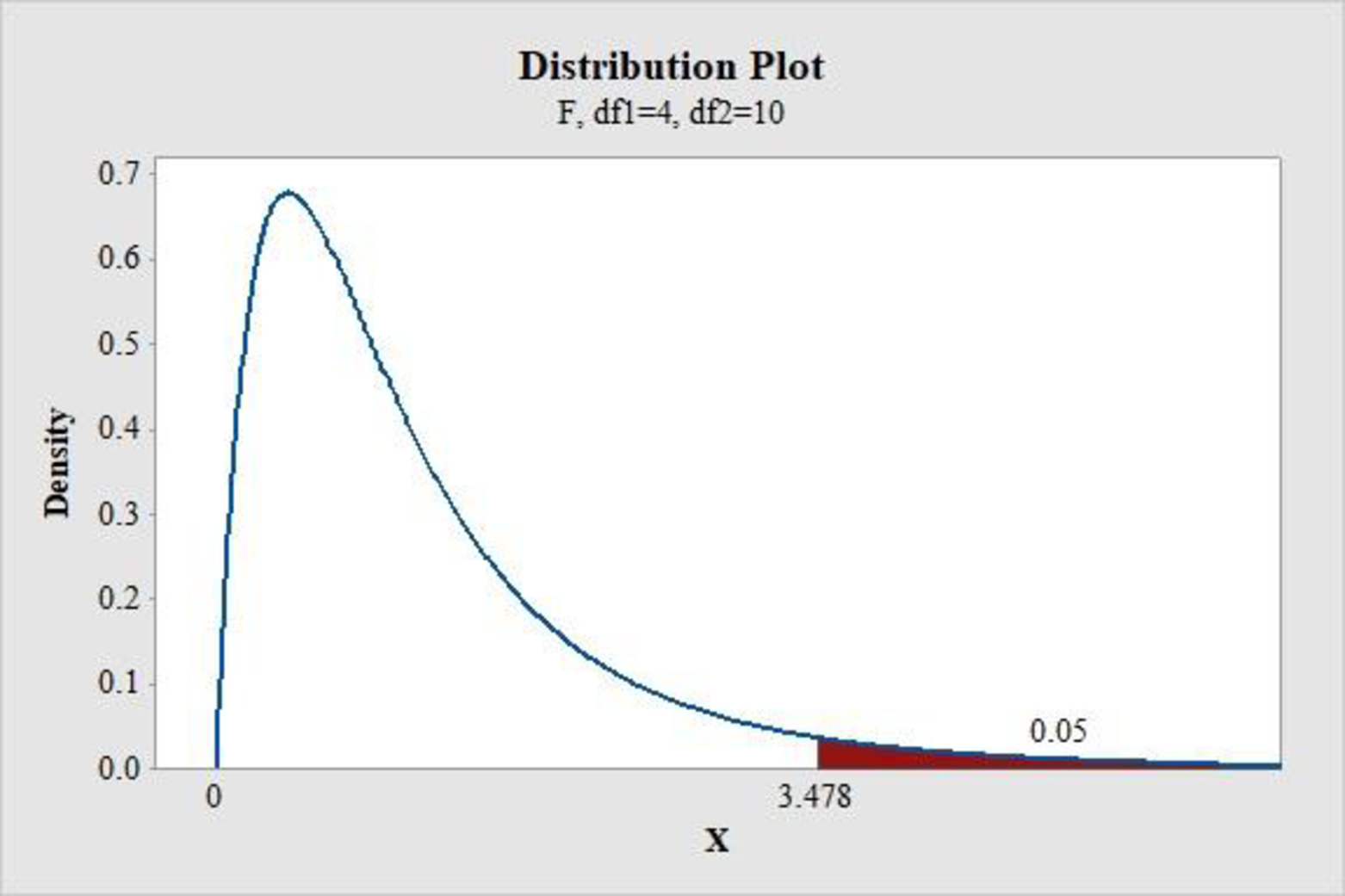
From the MINITAB output, the critical value is 3.478.
Conclusion:
If the F test statistic value is greater than the critical value, then reject the null hypothesis.
Therefore, the F test statistic of 16.2 is greater than the critical value of 3.478.
Hence, reject the null hypothesis.
Thus, there is convincing evidence that the model is useful.
For
The value of F test statistic is calculated as follows:
P-value:
Software procedure:
Step-by-step procedure to find the P-value using the MINITAB software:
- Choose Graph > Probability Distribution Plot choose View Probability > OK.
- From Distribution, choose ‘F’ distribution.
- Enter the Numerator df as 6 and Denominator df as 8.
- Click the Shaded Area tab.
- Choose Probability Value and Right Tail for the region of the curve to shade.
- Enter the Probability value as 0.05.
- Click OK.
Output obtained using the MINITAB software is represented as follows:

From the MINITAB output, the critical value is 3.482.
Conclusion:
If the F test statistic value is greater than the critical value, then reject the null hypothesis.
Therefore, the F test statistic of 12 is greater than the critical value of 3.482.
Hence, reject the null hypothesis.
Thus, there is convincing evidence that the model is useful.
For
The value of F test statistic is calculated as follows:
P-value:
Software procedure:
Step-by-step procedure to find the P-value using the MINITAB software:
- Choose Graph > Probability Distribution Plot choose View Probability > OK.
- From Distribution, choose ‘F’ distribution.
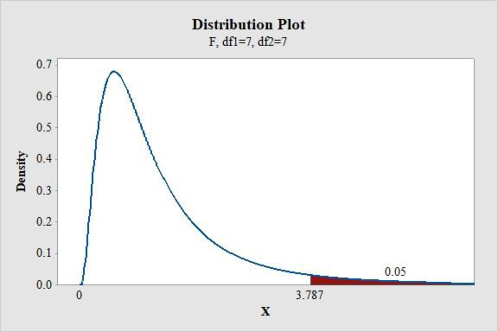
- Enter the Numerator df as 7 and Denominator df as 7.
- Click the Shaded Area tab.
- Choose Probability Value and Right Tail for the region of the curve to shade.
- Enter the Probability value as 0.05.
- Click OK.
Output obtained using the MINITAB software is represented as follows:

From the MINITAB output, the critical value is 3.581.
Conclusion:
If the F test statistic value is greater than the critical value, then reject the null hypothesis.
Therefore, the F test statistic of 9 is greater than the critical value of 3.581.
Hence, reject the null hypothesis.
Thus, there is convincing evidence that the model is useful.
For
The value of F test statistic is calculated as follows:
P-value:
Software procedure:
Step-by-step procedure to find the P-value using the MINITAB software:
- Choose Graph > Probability Distribution Plot choose View Probability > OK.
- From Distribution, choose ‘F’ distribution.
- Enter the Numerator df as 8 and Denominator df as 6.
- Click the Shaded Area tab.
- Choose Probability Value and Right Tail for the region of the curve to shade.
- Enter the Probability value as 0.05.
- Click OK.
Output obtained using the MINITAB software is represented as follows:
From the MINITAB output, the critical value is 3.787.
Conclusion:
If the F test statistic value is greater than the critical value, then reject the null hypothesis.
Therefore, the F test statistic of 6.75 is greater than the critical value of 3.787.
Hence, reject the null hypothesis.
Thus, there is convincing evidence that the model is useful.
For
The value of F test statistic is calculated as follows:
P-value:
Software procedure:
Step-by-step procedure to find the P-value using the MINITAB software:
- Choose Graph > Probability Distribution Plot choose View Probability > OK.
- From Distribution, choose ‘F’ distribution.
- Enter the Numerator df as 9 and Denominator df as 5.
- Click the Shaded Area tab.
- Choose Probability Value and Right Tail for the region of the curve to shade.
- Enter the Probability value as 0.05.
- Click OK.
Output obtained using the MINITAB software is represented as follows:
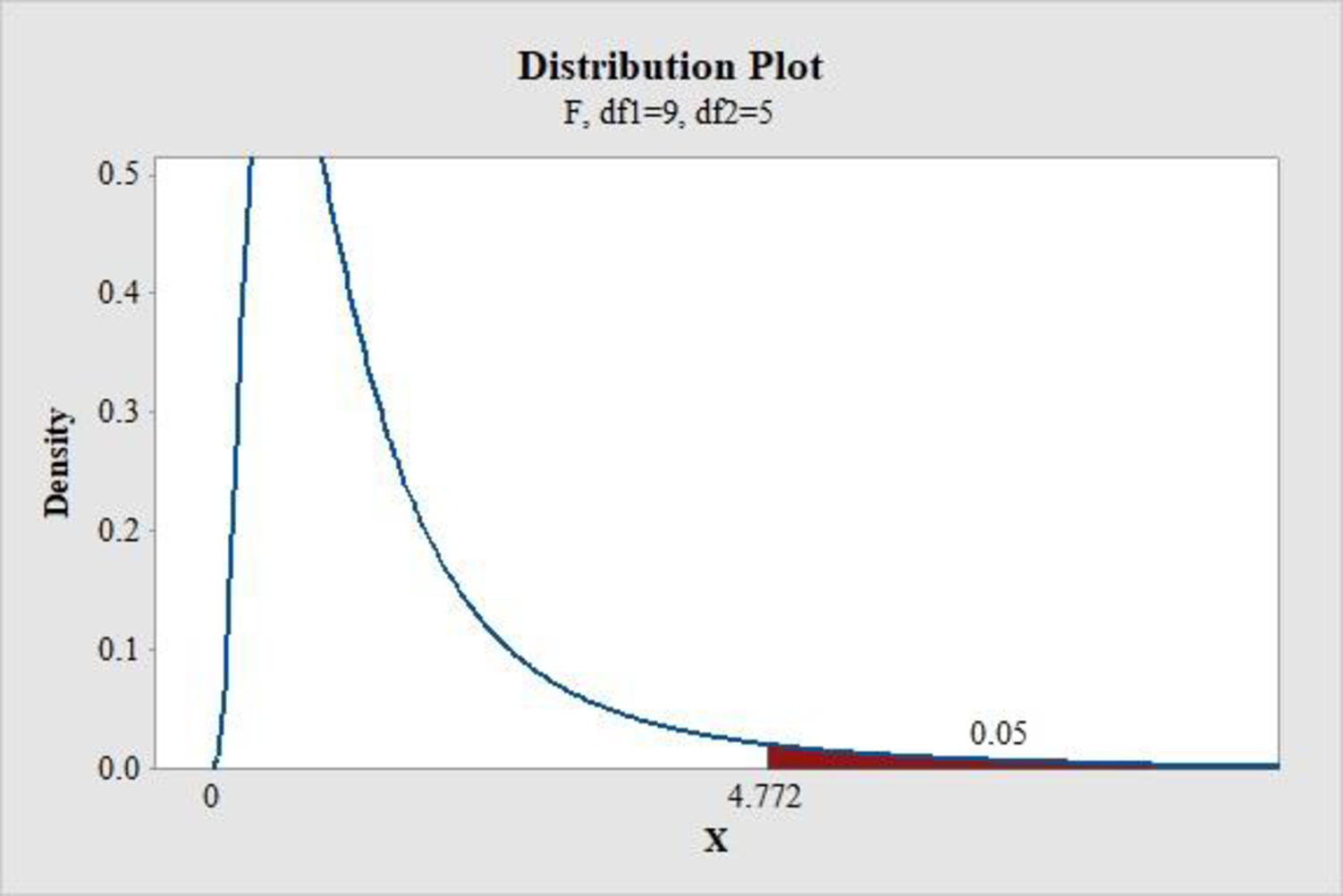
From the MINITAB output, the critical value is 4.772.
Conclusion:
If the F test statistic value is greater than the critical value, then reject the null hypothesis.
Therefore, the F test statistic of 5 is greater than the critical value of 4.772.
Hence, reject the null hypothesis.
Thus, there is convincing evidence that the model is useful.
For
The value of F test statistic is calculated as follows:
P-value:
Software procedure:
Step-by-step procedure to find the P-value using the MINITAB software:
- Choose Graph > Probability Distribution Plot choose View Probability > OK.
- From Distribution, choose ‘F’ distribution.
- Enter the Numerator df as 10 and Denominator df as 4.
- Click the Shaded Area tab.
- Choose Probability Value and Right Tail for the region of the curve to shade.
- Enter the Probability value as 0.05.
- Click OK.
Output obtained using the MINITAB software is represented as follows:
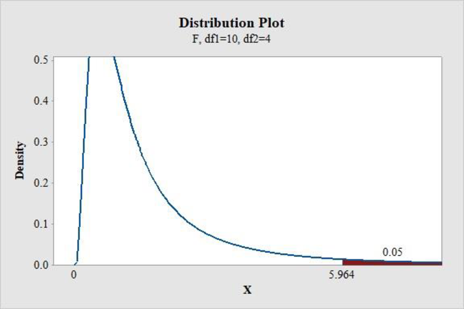
From the MINITAB output, the critical value is 5.964.
Conclusion:
If the F test statistic value is greater than the critical value, then reject the null hypothesis.
Therefore, the F test statistic of 3.6 is less than the critical value of 5.964.
Hence, fail to reject the null hypothesis.
Thus, there is convincing evidence that the model is not useful.
Conclusion:
For the value of k less than 9, there is evidence that the model is useful. For
Want to see more full solutions like this?
Chapter 14 Solutions
Introduction To Statistics And Data Analysis


 Linear Algebra: A Modern IntroductionAlgebraISBN:9781285463247Author:David PoolePublisher:Cengage Learning
 Glencoe Algebra 1, Student Edition, 9780079039897...AlgebraISBN:9780079039897Author:CarterPublisher:McGraw Hill