
Excel Applications for Accounting Principles
4th Edition
ISBN: 9781111581565
Author: Gaylord N. Smith
Publisher: Cengage Learning
expand_more
expand_more
format_list_bulleted
Videos
Textbook Question
Chapter 15, Problem 2R
The comparative financial statements of Global Technology are as follows:
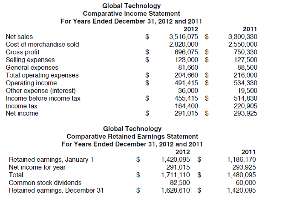
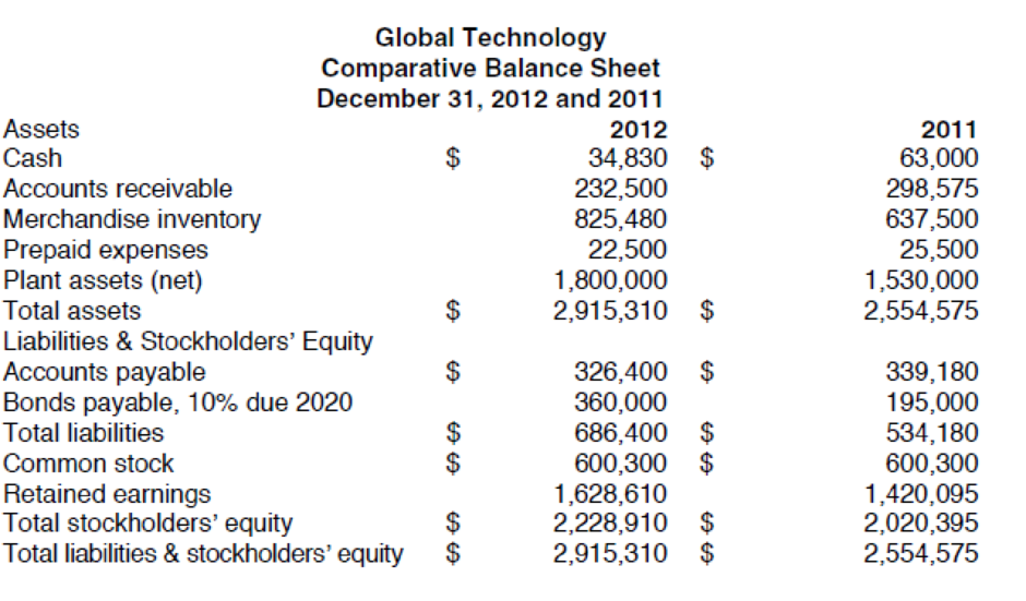
Open the file RATIOA from the website for this book at cengagebrain.com. Enter the formulas in the appropriate cells. Enter your name in cell A1. Save the completed model as RATIOA2. Print the worksheet when done. Also print your formulas. Check figure: Acid test (quick) ratio (cell C58), .82.
Expert Solution & Answer
Want to see the full answer?
Check out a sample textbook solution
Students have asked these similar questions
For the following five spreadsheet functions, (a) write the values of the engineering economy symbols P, F, A, i, and n, using a ? for the symbol that is to be determined, and (b) state whether the displayed answer will have a positive sign, a negative sign, or it can’t be determined from the entries. (1) = FV(8%, 10, 3000, 8000) (2) = PMT(12%, 20, –16000) (3) = PV(9%, 15, 1000,600) (4) = NPER(10%, –290,, 12000) (5) = FV(5%, 5, 500, –2000)
How difficult is it to expand the original RedBrandmodel? Answer this by adding a new plant, two newwarehouses, and three new customers, and modify thespreadsheet model appropriately. You can make up therequired input data.
Create an Income Statement for Till La Hok Computer Services. The other picture is just a sample for the format
Chapter 15 Solutions
Excel Applications for Accounting Principles
Ch. 15 - The comparative financial statements of Global...Ch. 15 - The comparative financial statements of Global...Ch. 15 - a. What information does a comparison of the...Ch. 15 - Prepare a ratio analysis for Global Technology for...Ch. 15 - Compare your printout from requirement 2 with your...Ch. 15 - With the 2013 data still on the screen, click the...
Knowledge Booster


Learn more about
Need a deep-dive on the concept behind this application? Look no further. Learn more about this topic, accounting and related others by exploring similar questions and additional content below.Similar questions
- JPL, Inc. has provided its sales and expense data for the most recent period. The Controller has asked you prepare a spreadsheet that shows the related CVP Analysis computations. Use the information included in the Excel Simulation and the Excel functions described below to complete the task.arrow_forwardUsing Excel, create a table that shows the relationship between the interestearned and the amount deposited, as shown. we will first create the dollar amount column and the interest row, as shown . Next we will type into cell B3 the formula = $A3*B$2. We can now use the Fill command to copy the formula in other cells, resulting in the table as shown. Note that the dollar sign before A3 means column A is to remain unchanged in the calculations when the formula is copied into other cells. Also note that the dollar sign before 2 means that row 2 is to remain unchanged in calculations when the Fill command is used.arrow_forwardFurther info is in the attached images For the Excel part of the question give the solutions in the form of the Excel equations. Please and thank you! :) Download the Applying Excel form and enter formulas in all cells that contain question marks. For example, in cell B34 enter the formula "= B9". After entering formulas in all of the cells that contained question marks, verify that the dollar amounts match the example in the text. Check your worksheet by changing the beginning work in process inventory to 100 units, the units started into production during the period to 2,500 units, and the units in ending work in process inventory to 200 units, keeping all of the other data the same as in the original example. If your worksheet is operating properly, the cost per equivalent unit for materials should now be $152.50 and the cost per equivalent unit for conversion should be $145.50. Thank you!arrow_forward
- The Excel worksheet form that appears below is to be used to recreate the Review Problem pertaining to the Magnetic Imaging Division of Medical Diagnostics, Inc. Download the workbook containing this form from Connect, where you will also receive instructions about how to use this worksheet form. You should proceed to the requirements below only after completing your worksheet. Required: 1. Check your worksheet by changing the average operating assets in cell B6 to $8,000,000. The ROI should now be 38% arid the residual income should now be $1,000,000. If you do not get these answers, find the errors in your worksheet and correct them. Explain why the ROI and the residual income both increase when the average operating assets decrease. 2. Revise the data in your worksheet as follows: a. What is the ROI? b. What is the residual income? c. Explain the relationship between the ROI and the residual income?arrow_forwardOne day, the company chooses to buy their new accounting information system (AIS), and decide which activities in the systems development life cycle (SDLC) can be skipped? Justify your choice and explanation.arrow_forwardFor this problem, there are 10 future value and present value exercises to be solved. Review the printout of the worksheet file COMPOUND that follows these requirements. This file also contains a second sheet called the Answer Sheet. Note that the worksheet is divided into four sections. You have to decide which section is appropriate for each exercise. Open the file COMPOUND from the website for this book at cengagebrain.com. To enter the four formulas in the appropriate cells, use the FV and PV functions for the annuities (see Appendix A in Excel Quick for a discussion of them). Unfortunately Excel does not provide functions for the future value of an amount nor the present value of an amount. Enter the following formulas for FORMULA1 and FORMULA2: FORMULA1: =B6*((1+B8)^B7) FORMULA2: =E6/((1+E8)^AE7) For the annuity calculations (FV and PV), it is important that you enter a value (or cell reference) for type to indicate the timing of the first payment. If the first payment is made…arrow_forward
- Below you will see three sets of inputs. After inputting all of your formulas, you should be able to use any of these sets of data and have the answers automatically update within excel. Please choose one of the data sets below and input all of the necessary formulas to find the answers. Once you are done, choose a different data set, enter it into your spreadsheet, and check the updated answers to ensure that everything is flowing through the formulas appropriately. A check answer for each one has been provided. Data set #1 Data Section: Actual and Budgeted Unit Sales: April 1,500 May 1,000 June 1,600 July 1,400 August 1,500 September 1,200 Balance Sheet, May 31, 19X5 Cash $8,000 Accounts Receivable 107,800 Merchandise Inventory 52,800 Fixed Assets (net) 130,000 Total assets $298,600 Accounts Payable (merchandise) $74,800 Owner's equity 223,800 Total liabilities & equity $298,600 Average selling price $98 Average purchase cost per unit $55 Desired ending inventory (% of next…arrow_forwardClick the Chart sheet tab. This chart is based on the problem data and the two income statements. Answer the following questions about the chart: a. What is the title for the X-axis? b. What is the title for the Y-axis? c. What does data range A represent? d. What does data range B represent? e. Why do the two data ranges cross? f. What would be a good title for this chart? When the assignment is complete, close the file without saving it again. Worksheet. The VARCOST2 worksheet is capable of calculating variable and absorption income when unit sales are equal to or less than production. An equally common situation (that this worksheet cannot handle) is when beginning inventory is present and sales volume exceeds production volume. Revise the worksheet Data Section to include: Also, change actual production to 70,000. Revise the Answer Section to accommodate this new data. Assume that Anderjak uses the weighted-average costing method for inventory. Preview the printout to make sure that the worksheet will print neatly on one page, and then print the worksheet. Save the completed file as VARCOSTT. Check figure: Absorption income, 670,000. Chart. Using the VARCOST2 file, fix up the chart used in requirement 5 by adding appropriate titles and legends and formatting the X- and Y-axes. Enter your name somewhere on the chart. Save the file again as VARCOST2. Print the chart.arrow_forwardMini Case Instructions Answer the following questions in a separate document. Explain how you reached the answer or show your work if a mathematical calculation is needed, or both. Mini Case Suppose you decide (as did Steve Jobs and Mark Zuckerberg) to start a company. Your product is a software platform that integrates a wide range of media devices, including laptop computers, desktop computers, digital video recorders, and cell phones. Your initial client base is the student body at your university. Once you have established your company and set up procedures for operating it, you plan to expand to other colleges in the area and eventually to go nationwide. At some point, hopefully sooner rather than later, you plan to go public with an IPO and then to buy a yacht and take off for the South Pacific to indulge in your passion for underwater photography. With these plans in mind, you need to answer for yourself, and potential investors, the following questions: What is an agency…arrow_forward
- Answer the following questions using the Answer Report and the Sensitivity Report on thefollowing page. Support your answers with explanations and the work showed.Your run a company that produces three electrical products – clocks, radios, and toasters. You are asked to figure out how many of each of these things should be produced, and the computer solution (answer report and sensitivity report generated in Microsoft Excel) is given on the next page. 1.) How many of each of the electronic appliances should you make? (Make sure your answer makes sense.)2.) How much will you end up profiting?3.) Which of the constraints are binding? What does the slack for each non-binding constraint represent?arrow_forwardFind the following values, using the equations, and then work the problems using a financial calculator to check your answers. Disregard rounding differences. (Hint: If you are using a financial calculator, you can enter the known values and then press the appropriate key to find the unknown variable. Then, without clearing the TVM register, you can "override" the variable that changes by simply entering a new value for it and then pressing the key for the unknown variable to obtain the second answer. This procedure can be used in parts b and d, and in many other situations, to see how changes in input variables affect the output variable.) Do not round intermediate calculations. Round your answers to the nearest cent. An initial $800 compounded for 1 year at 5.5%. $ An initial $800 compounded for 2 years at 5.5%. $ The present value of $800 due in 1 year at a discount rate of 5.5%. $ The present value of $800 due in 2 years at a discount rate of 5.5%. $arrow_forward1. Choose three of the following five technologies/techniques and explain why you think it is helpful in accounting analytics based on your lab experience in this course. Use some examples in your explanation. Limit your answer to 500 words in total. A. XBRL B. Tableau C. VLOOKUP function D. Pivot table E. Regressionarrow_forward
arrow_back_ios
SEE MORE QUESTIONS
arrow_forward_ios
Recommended textbooks for you
 Excel Applications for Accounting PrinciplesAccountingISBN:9781111581565Author:Gaylord N. SmithPublisher:Cengage Learning
 Essentials Of Business AnalyticsStatisticsISBN:9781285187273Author:Camm, Jeff.Publisher:Cengage Learning,
Excel Applications for Accounting Principles
Accounting
ISBN:9781111581565
Author:Gaylord N. Smith
Publisher:Cengage Learning
Essentials Of Business Analytics
Statistics
ISBN:9781285187273
Author:Camm, Jeff.
Publisher:Cengage Learning,
Topic 6 - Financial statement analysis; Author: drdavebond;https://www.youtube.com/watch?v=uUnP5qkbQ20;License: Standard Youtube License